Introduction
The problem of near-Earth environment congestion has become increasingly important due to the growing number of both active and inactive Resident Space Objects (RSOs), especially in Low-Earth Orbit(LEO). Traditionally, the problem of satellite tracking was handled by high-end sensors, such as radar tracking stations and telescopes, however, the appearance of low-cost, consumer level sensors such as Software-Defined Radios made it possible to introduce the network of low-cost ground stations that can assist the problem of tracking the population of orbiting objects.
When in operational state, the majority of satellites utilize several pre-defined frequency bands for beacon broadcasting and data transmission. When a satellite passes over an observer on the Earth’s surface, large relative velocity produces substantial Doppler shift relative to the emitted frequency. This project focuses on exploring methods for Initial Orbit Determination (IOD) based on Doppler and Doppler-related measurements obtained by a network of ground stations.
Approach
Due to the scale of the problem, one of the main challenges of IOD is the estimation of the approximate initial state vector that can then be refined through batch or sequential estimation methods, e.g. batch or Kalman filtering.
As the problem of state estimation through Doppler measurements and a single station is unobservable, i.e. it is impossible to infer the full state vector purely from Doppler or range rate observations, the need for multiple synchronized observing stations is required.
The overall approach can be divided in four main parts:
- Doppler shift and Time Differential of Arrival (TDoA) measurements
- Initial multilateration via TDoA
- Initial Orbit Determination using Herrick-Gibbs method
- Orbit estimate improvement through batch filtering
Background
Doppler Shift
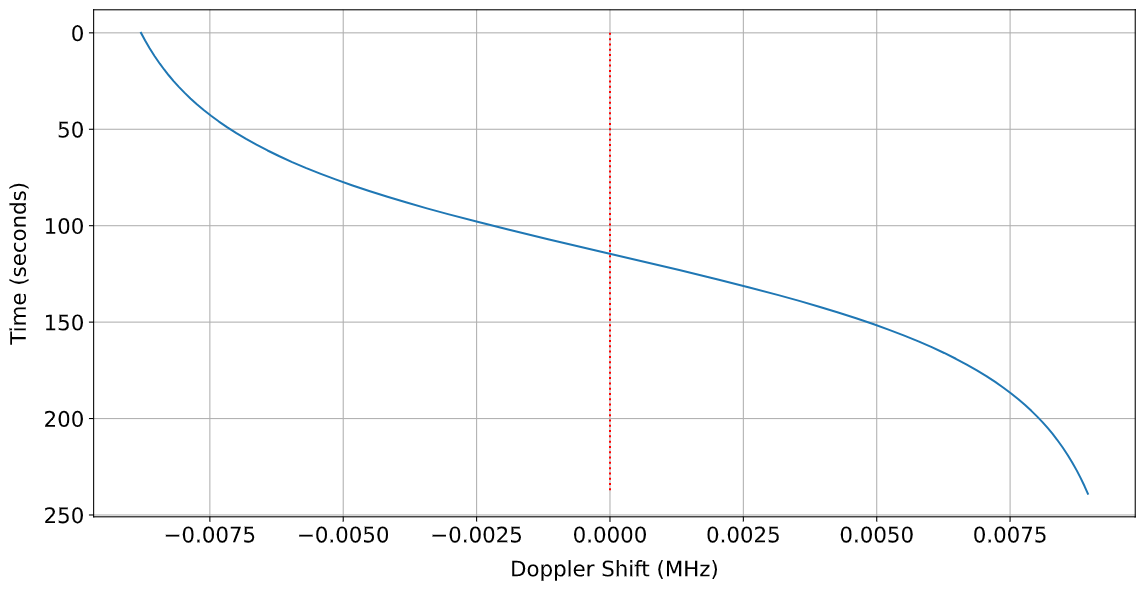
Doppler shift occurs due to the difference in velocity between emitter and observer and is directly proportional to the slant (line of sight) range rate. An example of Doppler shift is shown in Figure 1.
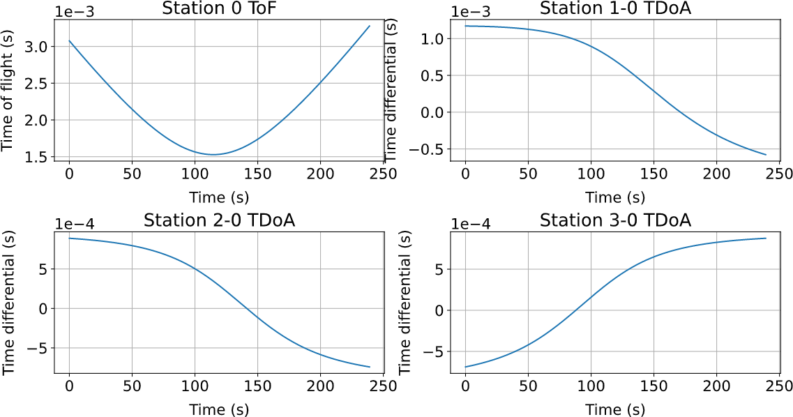
Time Differential of Arrival
When using multiple stations, it takes different amount of time for signal to travel from emitter to each of the station. The time difference in signal arrival is called Time Differential of Arrival (TDoA) and can be used to multilaterate the position of the emitter. In TDoA approach, observer positions are known while emitter position is the unknown variable to be found. The ranges between the observer and the emitter are determined using the estimate of the time it takes for signal to travel between the emitter and the observer In order to obtain the position estimate for the signal source, relative formulation of TDoA problem requires at least four stations (x,y,z positions and time offset) [3].
Herrick-Gibbs Initial Orbit Determination
Given short observation times between the consecutive measurements, Herrick-Gibbs IOD method is most suited for this problem. It calculates a velocity vector given three consecutive positional measurements with their corresponding timestamps. It uses Taylor series expansion to obtain a velocity vector for middle measurement. Consecutively, from three positional measurements a single full-state orbital estimate can be obtained, that can be further used as a separate measurement or initial estimate input for a sequential tracking method [2].
Batch Filter
Batch estimation filter is widely used in the problem of orbit determination. Unlike Kalman filter (while being mathematically equivalent to it) which is an on-line estimation algorithm, batch filter uses whole history of measurements to produce the best result for the initial state estimate. For more detailed explanation on batch filtering please refer to [1].
Proposed Approach
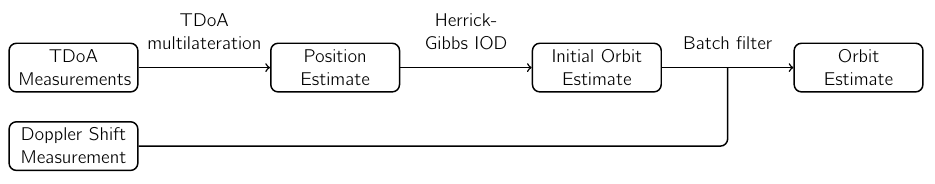
The general workflow of the proposed approach is shown in Fig. 3 and can be summarized as follows:
- Time differential and Doppler shift measurements are obtained through a synchronized network of stations. At least four stations are required as there are four unknowns.
- Approximate position estimate are obtained through multilateration of TDoA measurements. This step will provide us with position, but not velocity measurements, which are calculated in the next step.
- Velocity values are obtained through Herrick-Gibbs IOD providing rough initial orbital estimate.
- Initial orbit estimate is the used as a prior in batch filtering process.
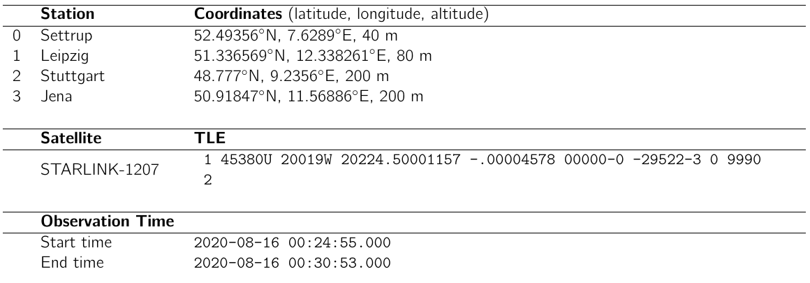
Simulation Scenario
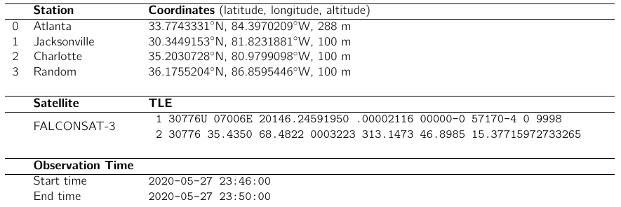
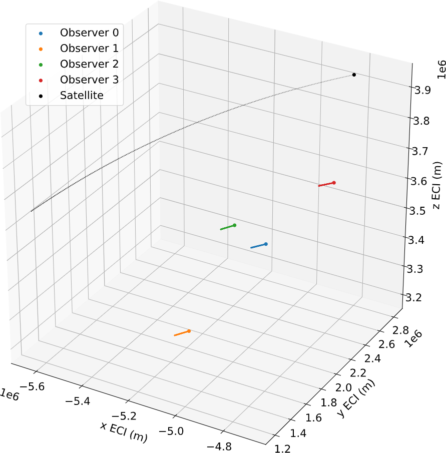
An example observation scenario has been created to test the validity of the proposed approach. The summary of the main example scenario used in this report is shown in Table. 1. Orbit was simulated for a amateur radio satellite with a given Two-Line Element (TLE). Graphical representation of the scenario is shown in Figure 4.
Results
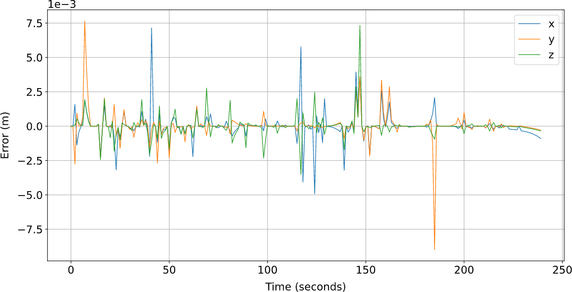
First, groundtruth satellite trajectory was used to simulate TDoA and Doppler shift measurements, as shown in Fig. 1 and 2. Then, the TDoA multilateration was performed for each timestep by solving the objective function using standard odeint solver. The position multilateration error is shown in Figure 5.
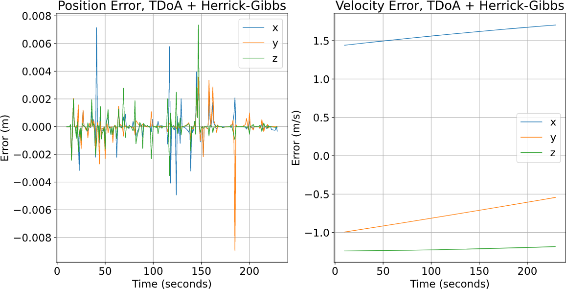
When combining TDoA solutions with Herrick-Gibbs IOD method, the resulting errors with respect to the groundtruth are shown in Figure 6.
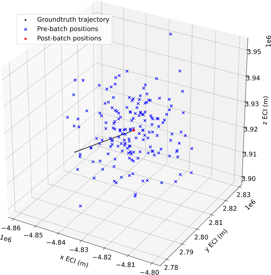
In order to show that despite the single station problem being unobservable, the Batch filter would still converge when the measurements are provided from several station, a Gaussian distribution around the initial groundtruth position of the satellite was used to sample 500 random samples, each being provided as a prior to the batch filter. The results are shown in Figure 7.
Results – Evaluation Simulation
In order to check the robustness and the validity of the proposed approach, a measurement file was provided by the organizer containing simulated measurements only, without any prior data. The summary of the evaluation simulation scenario is shown in Table 2.
In this case, initial TDoA multilateration showed the effect of Dilution of Precision – the farther and more in-line the satellite is with respect to the observers , the more difficult it is to multilaterate its position.
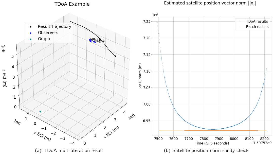
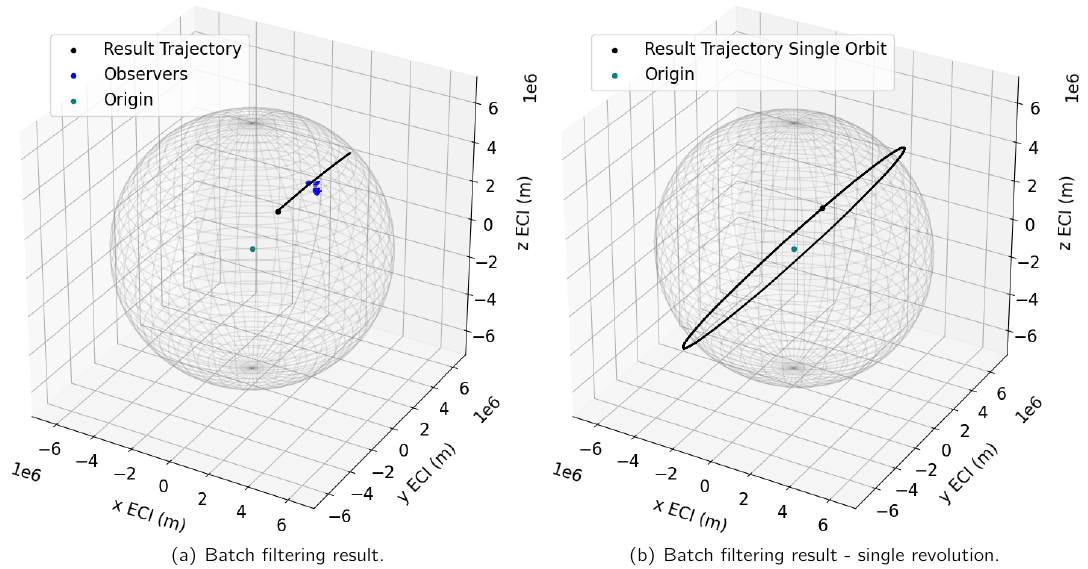
For the sake of simplistic representation, satellite position norm (norm of the position part of the vector) was used to show the uncertainty of the multilateration depending on the relative distance the closer it gets, the better the estimate is. When the estimate was provided to the batch filter, the measurements were trimmed to remove the worst positional estimates. The batch results are shown in Figure 9.
Conclusion
The initial results showed the viability of the proposed approach – given the two main challenges of problem observability and prior estimate, the algorithms were able to estimate the orbit of the satellite with no prior given Doppler shift and Time Differential of Arrival measurements.
Future work could include the improvement of the algorithm to handle noise and clutter as no real data is ideal as well as possibly incorporating additional approaches, such as frequency differential of arrival, and more comprehensive tracking algorithms, such as Unscented Kalman Filter.
Acknowledgements
I would like to thank Aerospaceresearch.net for providing me with opportunity to participate in Google Summer of Code 2020 as well as Google for making this program possible.
References
- Bob Schutz, Byron Tapley, George H. Born. Statistical Orbit Determination. Elsevier, 2004.
- D.A. Vallado. Fundamentals of Astrodynamics and Applications. Microcosm Press, 4th edition, 2013.
- Johny L Worthy III, Marcus J Holzinger. Uncued satellite orbit determination using signals of opportunity. AAS/AIAA Astrodynamics Specialist Conference, 2015.
Links
- Source Code/PR
- Notebook with code for final results
- Project Wiki – Batch Filter
- Project Wiki – Workflow
- LaTeX Report/Paper Draft
- andrey.pak@aerospaceresearch.net