[GSoC 21 | MOLTO3BP – MOLTO-IT-API | Mario R D]

Hello everyone !
My name is Mario Robert D’Ambrosio and I got selected for GSoC 21 with the University of Barcelona to work on the MOLTO-3BP and MOLTO-IT tracks.
During these weeks I had the pleasure to work with multiple mentors, Brandon Escamilla (brandon.escamilla@outlook.com) and Ginés Salar (100345764@alumnos.uc3m.es)
Our goals commitments were multiple: first and foremost to have an integrated working and refactored repository for the MOLTO-3BP (Refactor Github Link)

And to be able to yield a dynamic, yet simple frontend to consume for the University Carlos III (located in Madrid) students and whoever interested in understanding the dynamic amongst translunar orbits and trajectories.

This is why I worked closely with Brandon and Gines, both in charge respectively of mantaining the service accessible on the university’s server (Brandon) for the MOLTO-IT-API operations and the MOLTO-3BP (Gines).

Secondily, we decided also to focus on revamping the UI of the displayed results and moslty to encapsulate all the brilliant work done by Gines for his thesis into OOP modern factory pattern classes.
I chose a microservice approach, as a busy python programmer, I decided to go towards this route as microservices communications is easier to manage and mostly, it is the most prominent way to micro-architect projects in the 2021 dev era.

Work Roadmap

  • 1. Cleaning up the MOLTO-3BP Repository

First and foremost a cleanup of old files and unused files was done.

I cleaned nearly 30 files and removed many unused pieces of code

  • 2. Reformatting the MOLTO3BP Code

Next the code was architectured in small microservices that would allow for the orbits to be computed without incurring in extreme computational weight and or adding sophistication and Massive Controller strategy (https://github.com/uc3m-aerospace/MOLTO-3BP/pull/7/commits/a468244a0ac688391f5a2879f4e22f7759cb6ac0)

  • 3. Adding new running options

The running options were added as a runner in the python file and as static file
Also, clearly, a README was put to explain all the different layers of inputs.

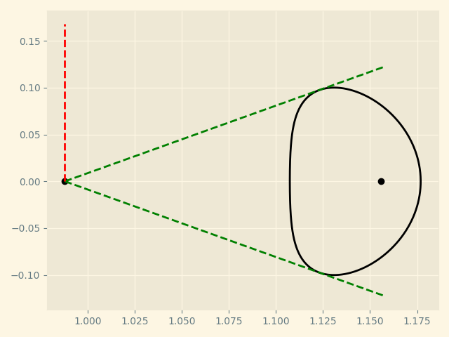
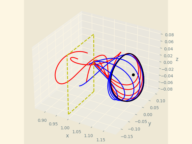
  • 4. Changing Image Layout

I have changed the layout in various sessions and offered custom plot graphic display

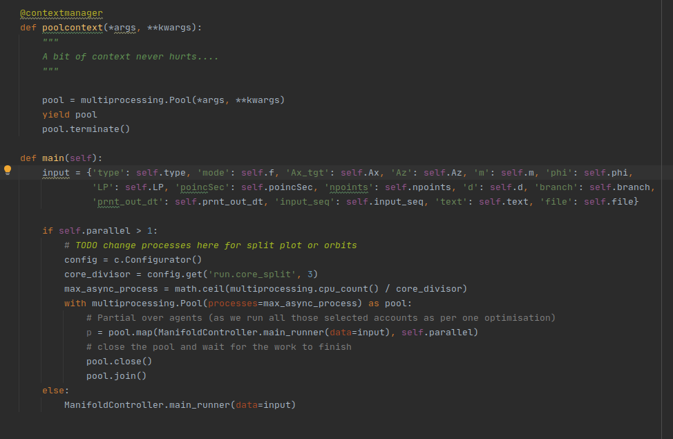
  • 5. Adding multiprocessing

Multiprocessing support for server and scalable core split was also added

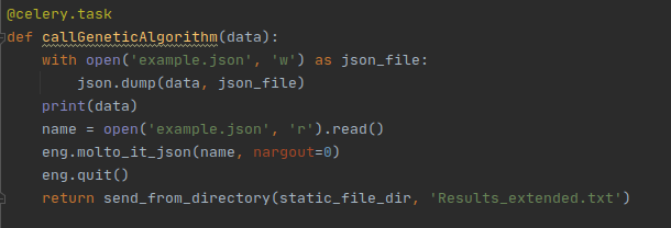
  • 6. Adding Flask Support

Finally, to consume the results as QUEUE and display the image with an interrogation system by JOB ID a Flask support was mandatory and added.
This would allow to consume the API and have the results ready asynchronously by calling with JOB ID

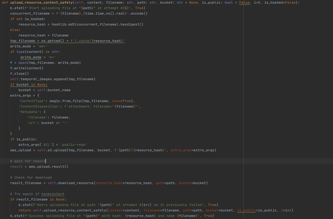
  • 7. Adding S3 resource saving support

I have added S3 Bucket support not to bloat the server and consume credits I’ve won on my AWS account in order to display the image results of plots continuously for students.
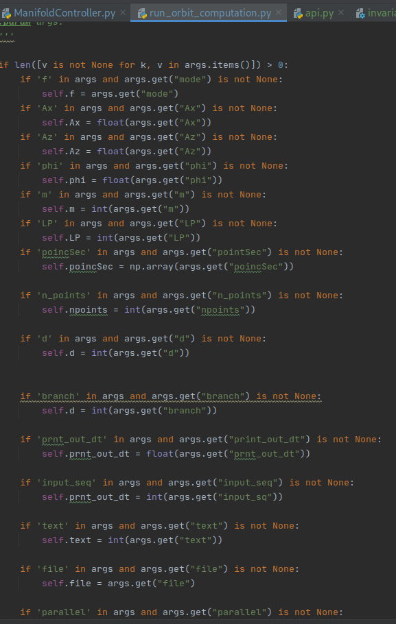
Snippets of code:

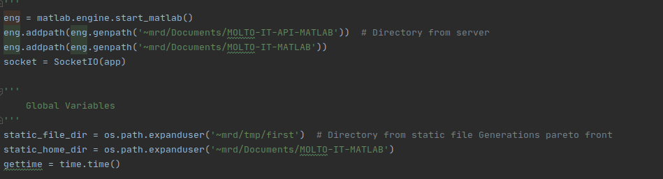
  • 8. Finally wrapping it into MOLTO-IT-API

Finally all the code was wrapped into MOLTO-IT, which needed some substantial repolishing and many features/packages upgraded in order for it to work.
Many code snippets were deprecated and, were thus, updated.
https://github.com/uc3m-aerospace/MOLTO-IT-API/pull/2/commits/8f4535e30023899f7a366507cacad533e721a025

Future work

Migration of API to FastAPI

As for the MOLTO-IT we would definitely like to expand and change some things.

Especially we would need to migrate the API to FastAPI to provide more flexibility and maintanance on the long run for the functions and portability.

Also genetic algorithm population and generations could be bettered calibrated to run in a case-specific solution scenario instead of just a plain global one.

This is going to be done by September – October 21 and could be finished in a new GSoC edition.


MAKING THE MOLTO-IT STATIC

It would be nice to dockerize and make the Molto IT static and folder/system agnostic, instead of having many code blocks hardcode as such

Lissajous Orbit

We also plan to work on the Lissajous orbit, which requires most of the computation, as it represents both a blend of the Lyapunov and Halo computations combined.
This is planned to be done by November – December 21.

Conclusion

I have learned so much from such experience, I would be capable of writing an essay for the enormous tasks learnt throughout such experience.

First, communication was essential for the deployment and delivery of the project.
Second, I learned about pacing myself and downplaying my expectations as to aiming high but delivering less is worse than aiming a bit lower and overdelivering.

I tried to aim at a not so fantasmagoric intention but have a GSoC plan and post GSoC plan.
My intentions were to being able to mantain and bring to life a repository where anyone could possibly contribute and deploy new open source code.

I think such intentions were achieved as we have now cleaned up a lot of code and created documentations (MOLTO-3BP -> https://github.com/uc3m-aerospace/MOLTO-3BP/pull/7/commits/0f3ca55a027e8541cc96d79956fbd1f98468116e, MOLTO -IT, MOLTO-IT -> https://github.com/uc3m-aerospace/MOLTO-IT-API/pull/2/commits/8f4535e30023899f7a366507cacad533e721a025)

As a Computer Engineer student, I have always shared a great passion for computer engineering problems and as an aerospace passionate, I enjoy amusing myself with astrophotography and amateur telescope obsevations.
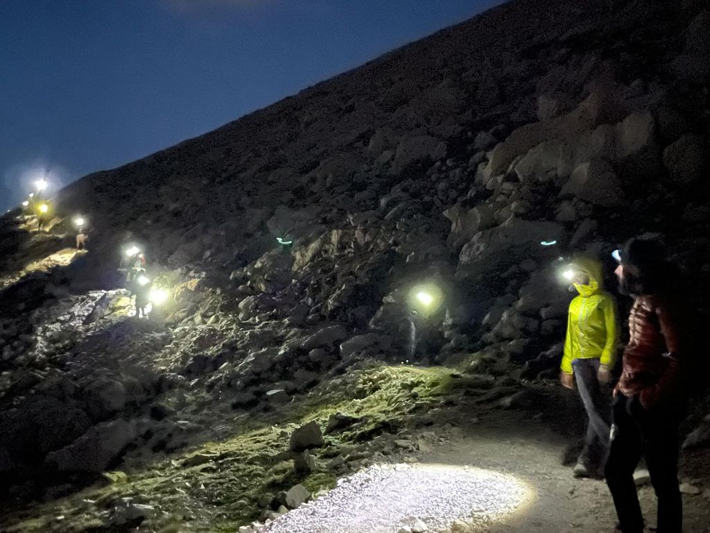
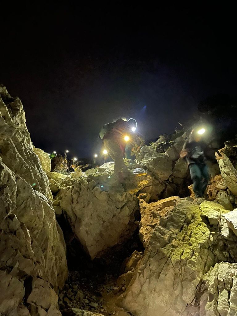
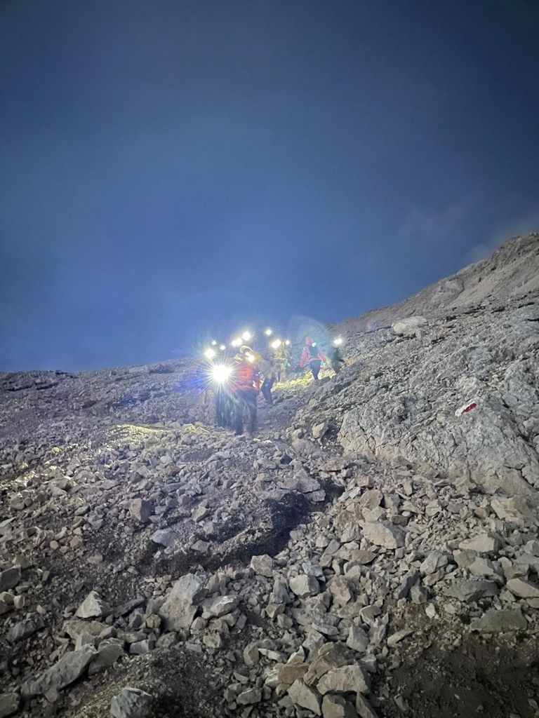
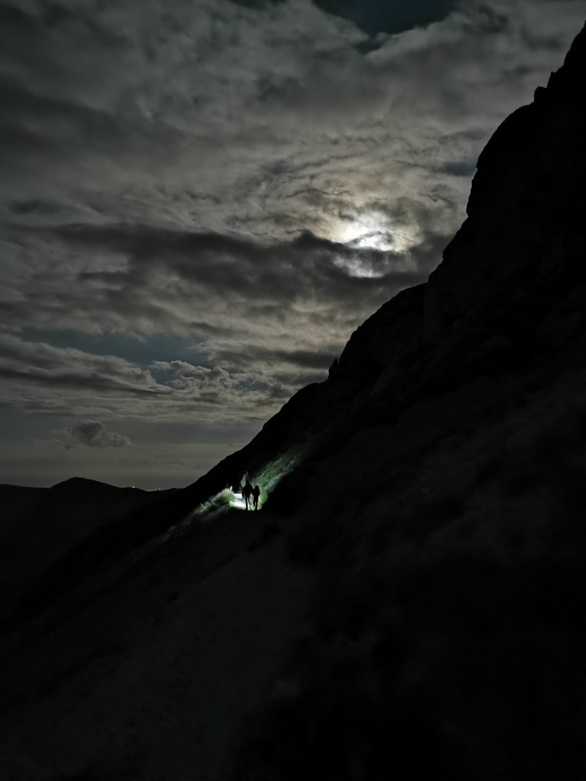
To close the GSoC 21 edition, I went and made my first ascent to the Corno Grande of Italy (https://en.wikipedia.org/wiki/Corno_Grande), where I went to the astronomical observatory and made a night climb to the peak (2912m) to challenge myself and close the GSoC edition with a bit of salt (and pepper! as this is not an easy hike/climb, experts only advised!).

I am grateful to have joined this GSoC edition and to be able to contribute in the future!

GSoC2021: Development of an FDIR algorithm using Neural networks

The goal of this project is to develop a failure detection, isolation and recovery algorithm (FDIR) for a cubesat, but using machine learning and neural networks instead of the more traditional methods.

Motivation: What is an FDIR algorithm and why is it usefull?

One of the most challenging parts of space missions is knowing and controlling where your spacecraft is, what is its relative orientation with respect to earth and how it is moving. Being aware of these three things is crucial to know if your spacecraft is flying too high or too low, too close to other spacecrafts, or simply if its oriented in a way that will allow it expose its solar panels to the sun to produce power or to point its antenna down to earth for calling home.

To perform this crucial task of computing and controlling its position and orientation spacecraft are designed with a variety of sensors and actuators that, together with proper control algorithms, ensure that your satellite remains where you want it and pointing in the right direction. This is often referred to as Attitude and Orbit control subsystem or AOCS.

Since this subsystem is critical for the spacecraft, it is needless to say that a failure in one of these sensors or actuators could easily kill your spacecraft and put and end to your mission. A faulty reading of a gyroscope that says that your spacecraft is rotating when it is not, a dead gyroscope that gives no signal and can’t tell if it is, or just a faulty thruster that provided more thrust than it should could leave your spacecraft spinning uncontrolled.

For these reason, providing the spacecraft on board software with a way of detecting these kind of failures as well as guidelines on how to proceed if one of these failures is detected is crucial for any space mission. This is done by means of the so called Failure Detection, Isolation and Recovery algorithms (FDIR).

Traditionally, these types of algorithms where simple, as they where based mainly on hardware redundancy , i.e., having many sensors that measure the same thing so that if one fails, you could detect the failure by looking at the rest and seeing that the signal is not consistent, isolate the failure by ignoring the reading from that sensor, and recover from the failure simply by continue to listen to the rest non-faulty sensors. While this is a valid and robust strategy to FDIR, it requires hardware redundancy of many spacecraft sensors and actuators, which means carrying on board more gyroscopes or reaction wheels than you actually need.

In recent years however, there has been a rising interest in low-cost space platforms such as Cubesats, pico or nano satellites that perform missions with much smaller budgets. One of the strategies used in these missions to reduce costs is to replace hardware based functionalities by software based ones, reducing therefore the number of components on board, the weight and power demands and overall complexity.

Replacing a hardware redundancy based FDIR strategy with a software based strategy is a perfect example of this. If your on board computer is capable of detecting a drift or a bias in the measurement of a sensor and correcting it without the need of comparing it with redundant sensors, or comparing it with the smallest number of redundant sensors possible then your mission might still be capable of safe operation, but minimizing the weight, power and cost penalties of hardware redundancy. There many ways to perform FDIR algorithms that focus on software instead of hardware, in order to explore some of the less conventional ones, it was decided to focus the project around machine learning and neural networks.

Project description

The goal of the project was then to set the basis of a neural network that could work to detect possible faulty signals from a cubestas sensors and actuators during its operation. This project had then two distinct lines of work:

  1. To develop or modify an existing simulator of a Cubesat to generate and extract the data from the sensors and actuators. This data is needed to train and test the Neural Network.
  2. To create an script capable reading and preprocessing the data from the simulator as well as creating, training and testing the neural network.

For the first, task an existing Cubesat simulator that included its own FDIR algorithm was used. This simulator written by Javier Sanz Lobo using Simulink included among its features the ability to simulate not only the cubesats motion, but also the readings from gyroscopes, reaction wheels and thrusters, as well as the capacity to induce artificial failures on the different components during the simulation. The original simulator can be found linked in the following repository:

https://github.com/msanrivo/SmallSat_FDIR

Several modifications where made to this simulator in order to fit it to it’s desired purpose. Among these it is worth highlihting:

  • The ability to Change the initial conditions to randomly generated ones within a desired range
  • A Matlab code that ran the simulator in a loop with random failure scenarios to generate the training and testing data
  • The capacity to export the readings from the sensors and actuators during the simulation to .txt files with the desired format.
  • Disabling the FDIR algorithm so that the simulated readings of the artificial failures remained unchanged.
  • The capacity of failures to occur at different times rather than at the start of the simulation.

For the second line of work, a scrip was written from scratch in python 3.8 using keras from the TensorFlow library to build, train and test the neural network. At the day of publishing this post, there are currently two scripts that read the data from 6 gyroscopes and 4 reaction wheels of the cubesat in the simulator and use one thousand simulations to train a Neural Network and a convolutional neural network. In both cases the network is then tested with another one hundred simulations to evaluate its real accuracy.

The end result is two types of neural networks that are both capable of predicting not only the most likely failure scenario that corresponds to that data, but also the probability of each individual failure scenario, which is a valuable input for future steps in the process of developing a fully functional FDIR algorithm.

Results

Currently both the traditional neural network and the convolutional one achieve accuracy values of around 70% in their predictions. Note that with 6 gyros and 4 Reaction wheels and the limitation of a maximum of two gyros and two reaction wheels failing the number of possible scenarios rises up to 242, which makes it hard to perform predictions.

Simpler scenarios where none of the devices fail are easily identified by both networks, as is the case of the following figure where both predict the correct outcome with a probability higher than 70%:

More complex scenarios where one or several devices fail reduce this prediction probability, making them capable of predicting correctly the failure of one device, but rarely all of them. In this cases, however, usefull information is provided by the probabilities, as the correct scenario can be found among those with the highest probabilities even if it is not the one with the highest.

Take for example the case depicted in the following figure where only one reaction wheel fails. The CNN is capable of predicting the correct scenario, but the NN predicts a scenario in which not only the aforementioned wheel fails, but also two complementary gyros as well. Note that even when predicting the wrong scenario, the NN shows the correct one as the second most likely.

Future work

A lot has been achieved during this GSoC period, yet there is still plenty of work ahead in this ambitious project. Among the features that are still to be implemented and tasks to be performed there are:

  • Continue to improve the neural networks to achieve better results at higher computational efficiencies.
  • Improve the simulator to generate better failure scenarios for thrusters.
  • Expand the FDIR capabilities of the network to include the simulated values of thrusters.
  • Research on reducing the number of input arguments to reduce the order of the problem and increase efficiency.
  • An interface between simulator and neural network to test and simulate in parallel.

Useful links

Github Repository: https://github.com/Rafabadell/FDIR_Neural_Networks

Author e-mail: Rafael.Badell@aerospaceresearch.net 

[GSoC2021: findsatbyrf] Center of satellite signal in the frequency domain

Overview:

This program finds the center in the frequency domain of a signal by time.

This is the link to its Github repository. There, you can also see the markdown (.md) file that contains the same content as this blog.

Every major work on this repository is done by Binh-Minh Tran-Huu under instructions and monitor from mentor Andreas Hornig of Aerospaceresearch.net as a project participated in Google Summer of Code 2021.

Usage:

Step 1: Prepare your wave file (.wav/.dat) and a json file containing the information about your signal

Example of the json file:

{
    "signal": {
        "name": "NOAA-18",
        "type": "NOAA",
        "center_frequency": 137.5e6,
        "time_of_record": "2021-06-04T20:17:05.00Z"
    },
    "tle": {
        "line_1": "1 28654U 05018A   21156.90071532  .00000084  00000-0  69961-4 0  9998",
        "line_2": "2 28654  98.9942 221.7189 0013368 317.9158  42.0985 14.12611611826810"
    },
    "station": {
        "name": "Stuttgart",
        "longitude": 9.2356,
        "latitude": 48.777,
        "altitude": 200.0
    },
    "default_channel": [
        {
            "frequency": 137912968,
            "bandwidth": 60e3
        }
    ]   
}

Where:

  • „signal“ object contains information about the signal file, such as name, center frequency and time of record. For now, there is only „type“: „NOAA“ is supported, if the signal is not NOAA then you should put „type“: null or simply remove that key.
  • „tle“ object contains the two lines of the „two-line element“ file of the satellite that the signal comes from.
  • „station“ object contains the information of the station, such as name, longitude (degree), latitude (degree) and altitude (meter).
  • „default_channel“ object contains a list of channels that will be analyzed in case there is no channel input from the command line. It could handle more than one channel, you can always add more channels into that list, for example:
"default_channel": [
        {
            "frequency": 400574.350e3,
            "bandwidth": 20e3
        },
        {
            "frequency": 400575.0e3,
            "bandwidth": 20e3
        }
    ]

NOTE: „tle“ and „station“ objects are only needed if you intend to use signal center frequency prediction based on TLE, „default_channel“ object is only needed if you want to not put channel information into the command line, otherwise you can remove them.

Step 2: Run the program from the Command-Line Interface (CLI)

Simply use Python to run the file main.py with the following arguments:

[-h] 
-f wav/dat_file 
-i json_file 
[-o name_of_output_file] 
[-ch1 frequency_in_Hz] [-bw1 frequency_in_Hz]
[-ch2 frequency_in_Hz] [-bw2 frequency_in_Hz]
[-bw3 frequency_in_Hz] [-ch3 frequency_in_Hz]
[-ch4 frequency_in_Hz] [-bw4 frequency_in_Hz] 
[-step time_in_second]
[-sen frequency_in_Hz] 
[-filter float]
[-tle] 
[-begin time_in_second]
[-end time_in_second]

With:

  • -h: to show help.
  • -f (required): to input the directory of the wave file.
  • -i (required): to input the json signal information file.
  • -o: directory and name without extension of the wanted output file, defaults to „./output“.
  • -ch0, -ch1, -ch2, -ch3: to input the frequencies (in Hz) of up to 4 channels to be analyzed. Will overwrite the „default_channel“ provided by the json file.
  • -bw0, -bw1, -bw2, -bw3: to input the bandwidth (in Hz) of up to 4 channels to be analyzed. Will overwrite the „default_channel“ provided by the json file.
  • -step: to input the length in time (in second) of each time interval, defaults to 1.
  • -sen: to input the sensitivity, which is the width of each bin in the frequency kernel (in Hz) after FFT, defaults to 1.
  • -filter: to input the strength of the noise filter as ratio to 1. For example, filter of 1.1 means the noise filter is 1.1 times as strong, or 10% stronger than the default filter, defaults to 1.
  • -begin: to input the time of begin of the segment to be analyzed, defaults to 1.
  • -end: to input the time of end of the segment to be analyzed, defaults to the end of the file.
  • -tle: used to turn on prediction based on Two-line elements (TLE) file, otherwise this function is off.

EXAMPLES:\

python3 .\main.py -i .\MySignal.json -f .\MySatellite\MySignal.wav -ch0 400.575e6 -bw0 20e3 -o D:\\CubeSat -begin 10. -end 60. -tle

python3 ./main.py -i /home/MyUser/MySignal.json -f ./MySatellite/MySignal.wav -ch0 400.575e6 -bw0 20e3 -o ./CubeSat

python3 ./main.py -i /home/MyUser/MySignal.json -f ./MySatellite/MySignal.wav -filter 1.25

Output:

  1. A time vs. frequency graph, showing the center of the signal in the frequency domain by time, for example: APT_NOAA example
  2. A .csv file storing the center position in the frequency domain by time.
  3. A .json file with a „header“ object containing metadata of the signal and „signal_center“ object containing centers of the signal for each channel by time.
  4. On the command-line interface, if -tle is enabled, there will be information about the offset between the calculated frequencies from the wave file and from the tle file as well as the standard error of the signal compared to prediction.

All files are exported with name and directory as selected with the [-o] argument.

Test files:

You can use the files here to test the code.

Description:

1. Introduction:

Because of the recent sharp growth of the satellite industry, it is necessary to have free, accessible, open-source software to analyze satellite signals and track them. In order to achieve that, as one of the most essential steps, those applications must calculate the exact centers of the input satellite signals in the frequency domain. My project is initiated to accommodate this requirement. It aims to provide a program that can reliably detect satellite signals and find their exact frequency centers with high precision, thus providing important statistics for signal analyzing and satellite tracking.

2. Overview

The project aims to locate the exact centers of given satellite signals with the desired accuracy of 1kHz, based on several different methods of finding the center. At first, the center-of-mass approach will be used to determine the rough location of the center. From that location, more algorithms will be applied depending on the type of the signal to find the signal center with higher accuracy. Currently, for many APT/NOAA signals, with the center-of-mass and “signal peak finding” approach (that will be shown below), we can get results with standard errors less than 1 kHz. For example, with the example signal above, the standard error is 0.026 kHz.

3. Theoretical basis

The overall flowchart: Flowchart

  • Fast-Fourier Transform (FFT)

Fourier Transform is a well-known algorithm to transform a signal from the time domain into the frequency domain. It extracts all the frequencies and their contributions to the total actual signal. More information could be found at Wikipedia: Discrete Fourier transform.

Fast-Fourier Transform is Fourier Transform but uses intelligent ways to reduce the time complexity, thus reducing the time it takes to transform the signal.

  • Noise reduction and background signal reset:
Noise in actual signal

In actual signals, there is always noise, but generally noise has two important characteristics, which is normally distributed and its amplitude does not change much by frequency. You can see the signal noise in the following figure:

If we can divide the signal in the frequency domain into many parts such that we are sure that at least one of them contains only noise, we can use that part to determine the strength of noise.

For example, consider only this signal segment:

One segment with noise

By taking its average, we can find where the noise is located relative to the amplitude 0. By subtracting the whole signal to this average, we can ensure the noise all lies around the zero amplitude.

One segment with noise

Next, we want to reduce all the noise to zero. To do that, we consider the distribution of noise, which is a normal distribution.

Normal distribution Photo from Characteristics of a Normal Distribution.

From this distribution, we are sure that 99.9% of noise has amplitude less than three times of the standard deviation of noise. If we shift the whole signal down by 3 times this standard deviation, 99.9% of the noise will have amplitude less than 0. From there, we can just remove every part of the signal with an amplitude less than zero. Then we will be able to get a signal without noise with the background having been reset to 0.

You can clearly see the effect of this algorithm by looking at the signal of PIXL1 satellite above, where all the noise has been shifted to below 0.

  • Center-of-mass centering

This algorithm is simple, the centroid position is calculated as: (sum of (amplitude x position)) / (sum of amplitude), similar to how we calculate the center of mass in physics. The result of this algorithm is called the spectral centroid, more information could be found at Wikipedia: Spectral centroid.

  • Peak finding.

For signals with clear peaks such as APT(NOAA), finding the exact central peak points of the signal would give us good results. From the rough location of the center by Center-of-mass method, we can scan for its neighbor to find the maximum peak. This peak will be the center of the signal that we want to find. For APT signals, this peak is very narrow, therefore this method is able to give us very high precision.

  • Predicted signal centers from TLE

TLE (Two-line element set) information of a satellite can be used to determine the position and velocity of that satellite on the orbit. By using this data of position and velocity, we can calculate the relativistic Doppler effect caused by the location and movement of the satellite to calculate the signal frequency that we expect to receive on the ground. For more information, visit Wikipedia: Relativistic Doppler effect.

  • Error calculation. Assume TLE gives us the correct result of signal center, we can calculate the standard error of the result by calculating the standard deviation:
Standard deviation

Where n is the number of samples, x_i is the difference between our calculated center frequency from .wav and the frequency we get from TLE.

4. Implementation in actual code:

  • main.py is where initial parameters are stored. The program is executed when this file is run.
  • tracker.py stores the Signal object, which is the python object that stores every information about a signal and the functions to find its center.
  • tools.py contains the functions necessary for our calculation, as well as the TLE object used for center prediction.
  • signal_io.py stores functions and objects related to the input and output of our signals and instructions.

5. Current results:

  1. For APT(NOAA): Standard error = 0.004 kHz APT_NOAA example
  2. For PIXL1(CUBESAT): Standard error = 0.029 kHz PIXL example

6. Potential further improvements:

  • Expand the program to work better with more types of signals.
  • Make video-output function works with reasonable computing resources.
    Currently, with my private version of the code, I am able to make videos such as this one, but it took too much time and memory to actually make one, therefore I did not put it into the official code.

[GSoC2021] CalibrateSDR GSM Support

Overview

CalibrateSDR developed by Andreas Hornig, is a tool developed to determine the frequency drift of Software Defined Radios precisely using sync pulses of various Signal Standards.  

Cheaper SDRs use a low-quality crystal oscillator which usually has a large offset from the ideal frequency. Furthermore, that frequency offset will change as the dongle warms up or as the ambient temperature changes. The result is that any signals received will not be at the correct frequency, and they would drift as the temperature changes. CalibrateSDR can be used with almost any SDR to determine the frequency offset.

The work on GSM (2G) has been done by Jayaraj J, mentored by Andreas Hornig, as part of Google Summer of Code 2021, the working directory for the same can be found at Github.

proposed working of CalibrateSDR – made GSM signal compatible (the below guide shows how to get started)

Project Description

GSM uses time division to share a frequency channel among users. Each frequency is divided into blocks of time that are known as time-slots. 8 time-slots are numbers TS0 – TS7. Each time slot lasts about 576.9  μs. The bit rate is 270.833 kb/s, a total of 156.25 bits can be transmitted in each slot.

Each slot allocates 8.25 of its „bits time“ as guard-time, split between the beginning and the end of each time slot. Data transmitted within each time slot is called a burst. There are several types of bursts.

Frequency correction burst is a burst of a pure frequency tone at 1/4th the bitrate of GSM or (1625000 / 6) / 4 = 67708.3 Hz. By searching a channel for this pure tone, we can determine its clock offset by determining how far away from 67708.3Hz the received frequency is.

How is it working?
  1. Scanning of GSM Channels is based on the ARFCN frequency bands. For tuning into GSM Frequency, the ARFCN script can be used. We give the input of band to scan, the result will be the frequency. If we input the „scan all“ option, it will scan the whole GSM Frequencies in the given band and return the offset calculated from each frequencies. The code for the same can be found at: https://github.com/aerospaceresearch/CalibrateSDR/blob/jyrj_dev/calibratesdr/gsm/arfcn_freq.py
  2. After scanning channels in specific bands using ARFCN, the program will record the sample in the given sample rate. Make sure the SDR is connected with the device, or we can record it and give the input as a wave file.
  3. The determination of the position of FCCH bursts that we receive in SDRs is done by the code in fcch_ossfet.py. We measure it by how much shifted is the FCCH burst, than what we expect, that is at 67708.3 Hz from the frequency centre. Simply, if no offset is there, we could see these tone bursts at 67708.3 Hz offset concerning the centre frequency of the channel.
  4. The final output we receive include
    • Frequency drift from the expected FCCH position
    • The Offset of SDR in PPM
  5. The whole code works from the main cali.py and inturns gsm.py files
To test with the IQ_file.wave:

After cloning the repo locally, run the setup to install the requirements using the command: python setup.py install

After that, to run the visualization plots, run:

python cali.py -m gsm -f <location of wav file> -rs <sampling rate> -fc <frequency center>

First, we will get the plot of the average power spectrum plot. Play with the code to increase the N value, and you can see the sharpness of the line.

Further plots generated includes TDMA frames, the position of FCCH bursts visualisation as given below.

Screenshot-spectrogram_hann-Zoomed.png

We can see the pure tone FCCH bursts are occurring at specific intervals and can be visualized as small blue dots at a range of 0.25 from the centre.

Thus implementation of a filter bank and calculating the positions of these FCCH bursts will give us the offset frequency since we know these FCCH bursts occur at a distance of 67708.3 Hz from the frequency centre.

The average power spectrum of Discrete Fourier Transforms

Usage

Test files for GSM, recorded by Andreas can be found here.

  • Setup the environment, make sure the requirements are installed (preferably in a virtualenv). Use the setup.py to install necessary requirements.
  • To view the parameters for input run ~$ python cali.py -h

usage: cali.py [-h] [-f F] [-m {dab,dvbt,gsm}] [-s {rtlsdr}] [-c C] [-rs RS] [-rg RG] [-rd RD] [-nsec NSEC] [-gr] [-v] [-fc FC]

optional arguments:
-h, –help show this help message and exit
-f F select path to input file
-m {dab,dvbt,gsm} select mode
-s {rtlsdr} scan with rtlsdr
-c C scan by „all“ channels, by channel number „0,1,…n“ or by block name
-rs RS file/scan sample rate
-rg RG scan with gain
-rd RD scan with the device
-nsec NSEC scan for n-seconds
-gr, –graph activate graphs
-v, –verbose an optional argument
-fc FC frequency centreSetup the environment, make sure the requirements are installed (preferably in a virtualenv). Use the setup.py to install necessary requirements.

  • If testing with a recorded wav file, enter the parameters as:
~$ python cali.py -m gsm -f <location of wav file> -rs <sampling rate> -fc <frequency center>
  • If testing with an SDR stick, specify the ARFCN band, or specific frequency centre to scan for the GSM channel.

The ARFCN Bands include: GSM_850, GSM_R_900, GSM_900, GSM_E_900, DCS_1800, PCS_1900. For more information about the arfcn, checkout here.

Example usage:

~$ python cali.py -m gsm -s rtlsdr -c 900

The above parameters can be changed according to user needs. -rs can be specified with sample rate. The exact sample rate will be shown with the result. Make sure the SDR is connected when running the code with -s rtlsdr argument. Specify the -fc frequency argument, if the scan is to be done with a single frequency.

The expected output would look like this:

{'f': None, 'm': 'gsm', 's': 'rtlsdr', 'c': '900', 'rs': 2048000, 'rg': 20, 'rd': 0, 'nsec': 10, 'graph': False, 'verbose': False, 'fc': None}
let's find your SDR's oscillator precision
scanning…
starting mode: gsm
Found Rafael Micro R820T/2 tuner
Exact sample rate is: 270833.002142 Hz
Scanning all GSM frequencies in band: GSM_900
Offset Frequency: 31031.66666666667
Offset in PPM: 33.179448397684716

The Offset calculated from the frequency drift between fcch positions can be precisely derived and can be used to correct the oscillator.

Potential further improvements:
  1. LTE Signal support need to be included (currently in focus), and much more standards need to be made compatible for a wide usage of the tool.
  2. Making a platform-neutral API to communicate with more SDR devices.
  3. Optimising the user interface (command-line tool can be made more user friendly).

References:

Find out the project updates in my branch and do give a star for the project in AerospaceResearch org:

https://github.com/aerospaceresearch/CalibrateSDR/tree/jyrj_dev

[GSoC’21 : Calibrate-SDR] DVB-T for calibration

Overview :

This project helps in calculating the frequency offset cause by heating of local oscillators of your SDR (Software Defined Radio) using some reference signals like DAB+, GSM, DVB-T, etc.

Link to its GitHub Repository.

This project is extended by Ayush Singh under the guidance of Andreas Hornig as mentor from AerospaceResearch.net as a project in Google Summer of Code.

Usage of Tool :

  • Clone the GitHub Repository to your local machine.
  • Run the setup.py
  • Once setup is done. Follow this –

Now you know the PPM shift of your device. You can now use it to do bunch of different things with you SDR.

ALL THE BEST for your project.