[GSoC2018|OrbitDeterminator|Jorge] Angles-only orbit determination: Gauss method and least-squares

1. Introduction

During GSoC 2018, I worked on developing a ra/dec angles-only Keplerian orbit determination implementation for AerospaceResearch.net’s orbitdeterminator project. Our implementation incorporates both elements from the Gauss method for orbit determination, as well as from the least-squares principle. I did this both for Earth-orbiting bodies (satellites, space debris, etc.), and Sun-orbiting bodies (asteroids, comets, centaurs, etc.).

My implementation makes use of the astropy library, whose SkyCoord class provided the adequate abstraction in order to perform the required computations. astropy was also really useful for handling of units, angles, longitudes, etc., as well as providing access to the SPK kernel of JPL ephemerides DE432s, which are at the core of the orbit determination for Sun-orbiting bodies. Also, the poliastro library was useful for the evaluation of Stumpff’s functions in order to perform the refinement stages of the Gauss method. Finally, scipy’s functionality allowed the use of the Levenberg-Marquardt method for the least-squares fit to ra/dec observations.

2. Link to my GSoC 2018 project work:

The main part of the work I did is contained in the following modules:

  • orbitdeterminator/kep_determination/gauss_method.py
  • orbitdeterminator/kep_determination/least_squares.py

The pull request associated to my GSoC project is in GitHub at: aerospaceresearch/orbitdeterminator PR #141. My GitHub handle is @PerezHz . You can also find me on Twitter as @Perez_Hz.

3. Gauss method

The orbitdeterminator/kep_determination/gauss_method.py module allows the user to input files which contain ra/dec observations of either Earth-orbiting or Sun-orbiting celestial bodies, following specific formats for each case, and allows to compute an orbit from n>=3 observations.

If the number of observations is n==3, then the Gauss method is applied to these 3 observations. Otherwise, if n>3, then the Gauss method is executed over n-2 consecutive observation triplets. A set of orbital elements is computed for each of these triplets, and an average over the resulting n-2 set of elements is returned. A refinement stage has been implemented for the Gauss method such at each iteration of the refinement stage, a better approximation for Lagrange’s f and g functions are computed; which in turn allows to get better estimates for the cartesian state of the observed body.

The right ascension and declination observations topocentric, i.e., they are referred to registered sites either by the MPC or COSPAR. The information about the geocentric position of these sites is contained in registered lists. Both the IOD and MPC formats contain the alphanumeric codes associated to each observation site, so that for each observation it is possible to compute the geocentric position of the observer. This whole process is automatically processed during runtime in the background, so the user does not need to worry about these details.

3.1 Earth-orbiting bodies: gauss_method_sat

The gauss_method_sat function computes Keplerian elements from ra/dec observations of an Earth-orbiting body. The call signature is the following:

gauss_method_mpc(filename, bodyname, obs_arr, r2_root_ind_vec=None, refiters=0, plot=True)

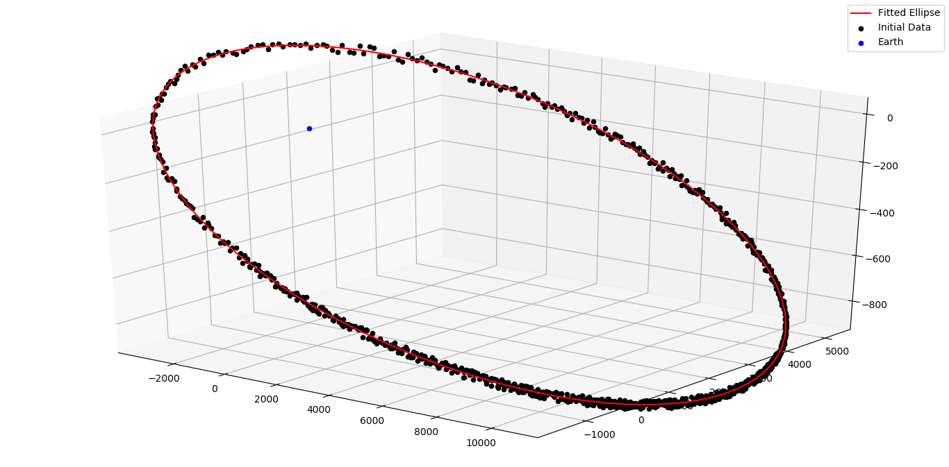
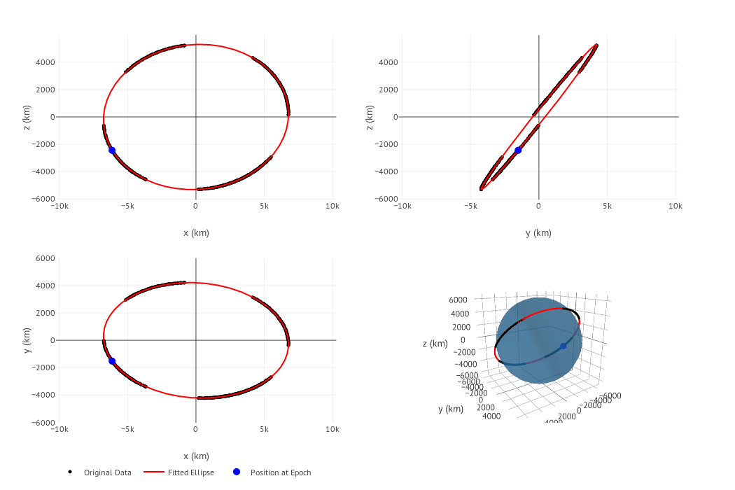
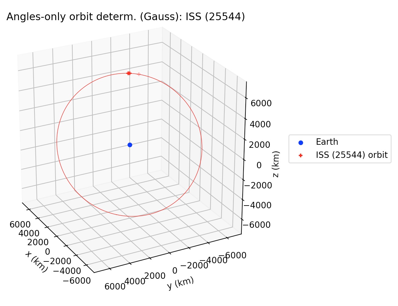
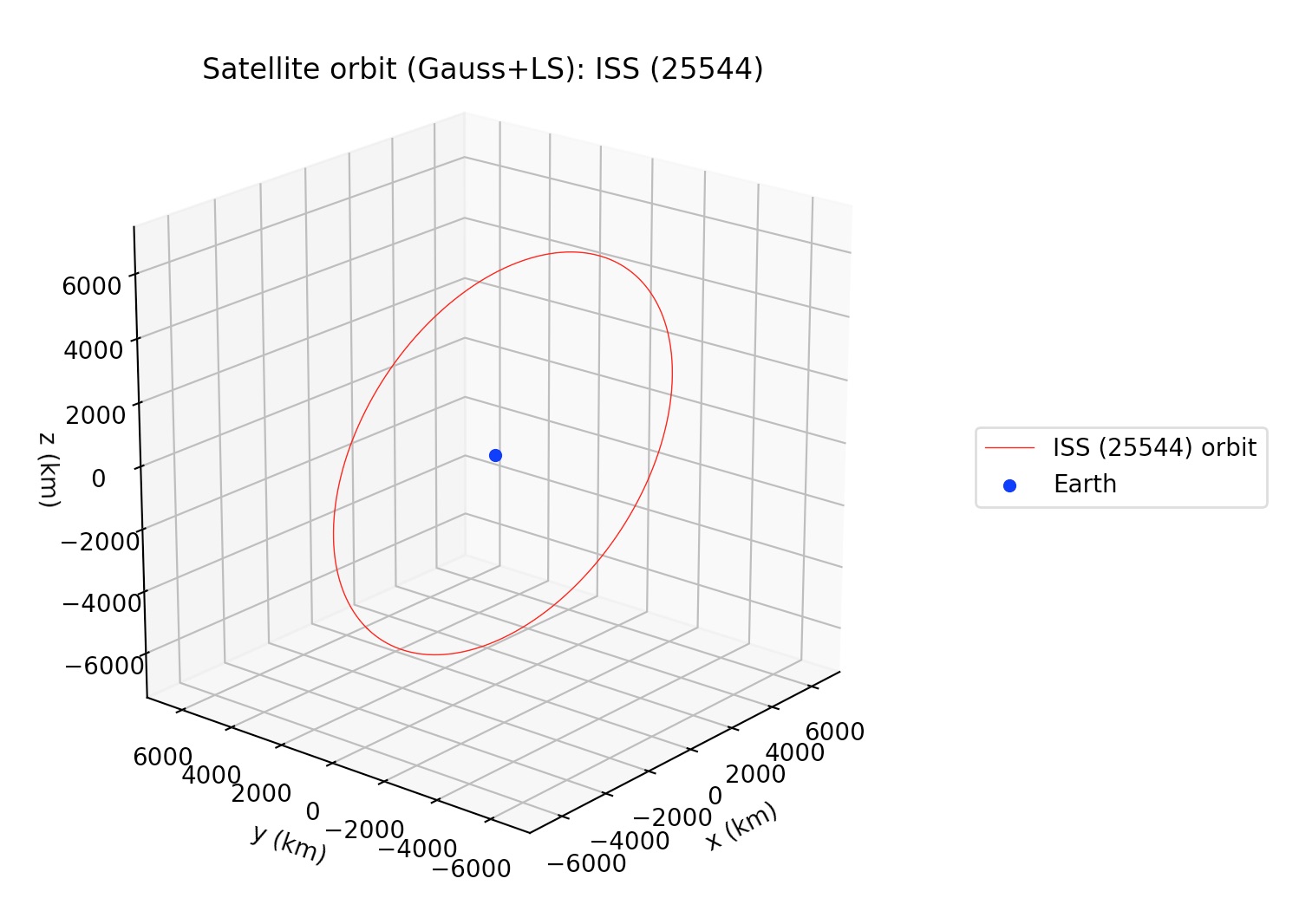
Where filename refers to the name of the file which contains the observations in IOD-format, bodyname is an user-defined name for the observed object, obs_arr is a list/array of integers which define the numbers of the lines in the observation file filename which are going to be processed, r2_root_ind_vec allows the user to select the roots whenever multiple solutions to the Gauss polynomial exist (default behavior is to select always the first root), refiters is the number of iterations for the refinement stage of the Gauss method (default value is 0), and plot is a flag which if set to True will plot the orbit of the object around the Earth. More details may be found at the examples and the documentation. The orbital elements are returned, respectively, in kilometers, UTC seconds and degrees, and they are referred to the (equatorial) ICRF frame. More details may be found at the examples and the documentation.

Example output:

3.2 Sun-orbiting bodies: gauss_method_mpc

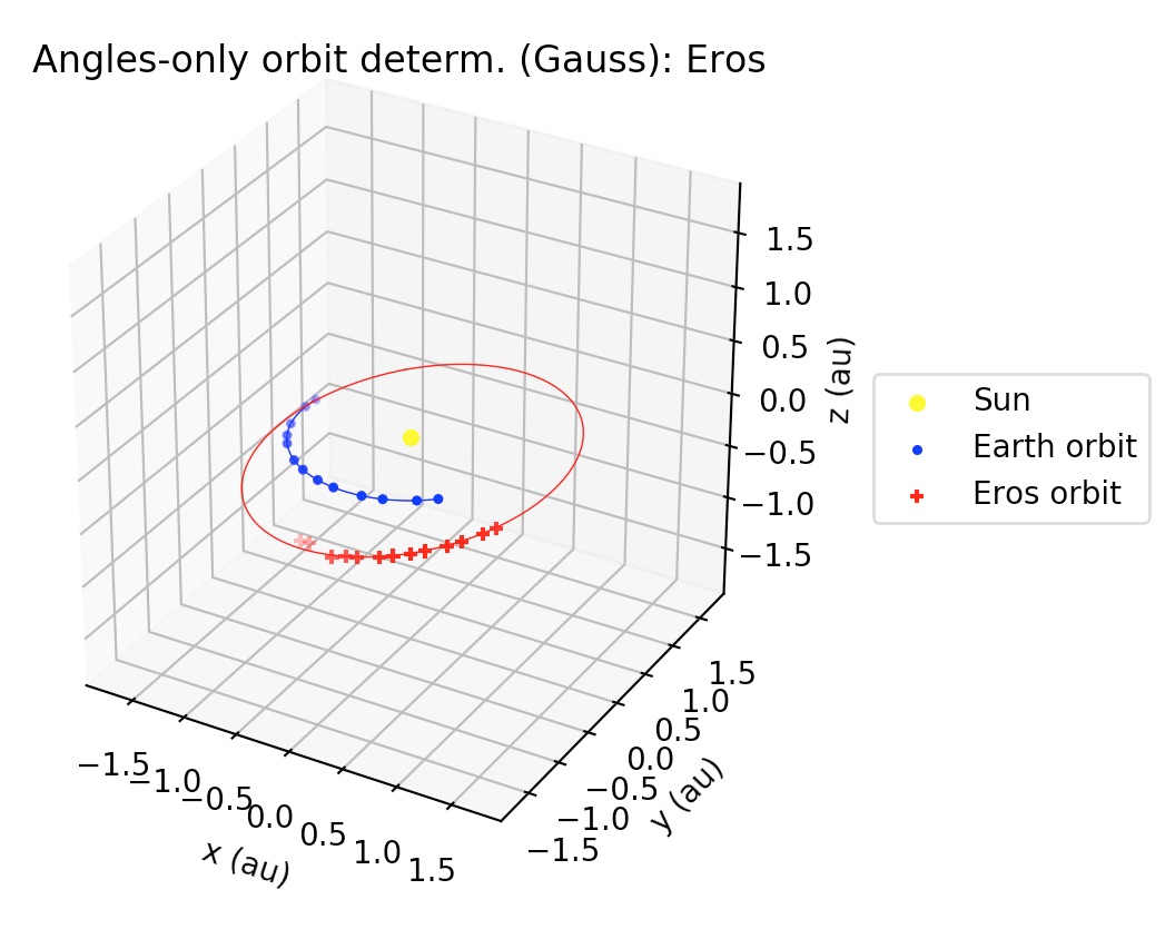
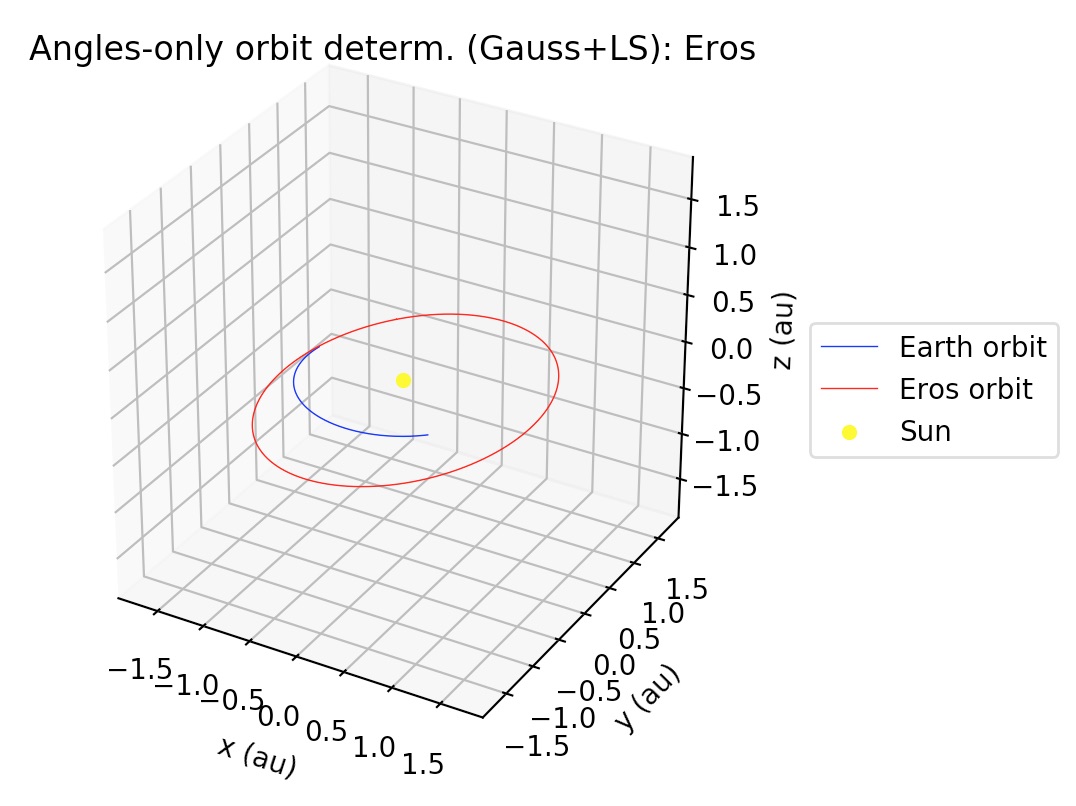
The gauss_method_mpc function computes Keplerian elements from ra/dec observations of an Earth-orbiting body. The call signature is practically same as gauss_method_sat (see section 3.1). One of the differences with respect to the Earth-orbiting case is that in this case the orbital elements are returned, respectively, in astronomical units, TDB days and degrees. But the main difference in the internal processing is that in this case, since the orbit is referred to the Sun, then the position of the Earth with respect to the Sun has to be determined at each of the observation times. gauss_method_mpc uses the JPL DE432s, as provided by the astropy library, in order to compute the heliocentric position of the Earth. This also involves a conversion from the UTC to the TDB time scale, which is also handled again using astropy’s time scale conversion functionalities. Finally, a third difference is that Sun-orbiting orbital elements are returned in the mean J2000.0 ecliptic heliocentric frame. More details may be found at the examples and the documentation.

Example output:

4. Least-squares

The least-squares functionality developed during my GSoC project may be thought of as differential corrections to the orbits computed by the Gauss method. That is, once a preliminary orbit has been determined by the Gauss method, then the best-fit of the observations to a Keplerian orbit in terms of the observed minus computed residuals (the so-called O-C residuals) may be found by a least-squares procedure. It is worthwhile to mention that in the current implementation all the observations have the same weight in the construction of the O-C residuals vector.

4.1 Earth-orbiting bodies: gauss_LS_sat

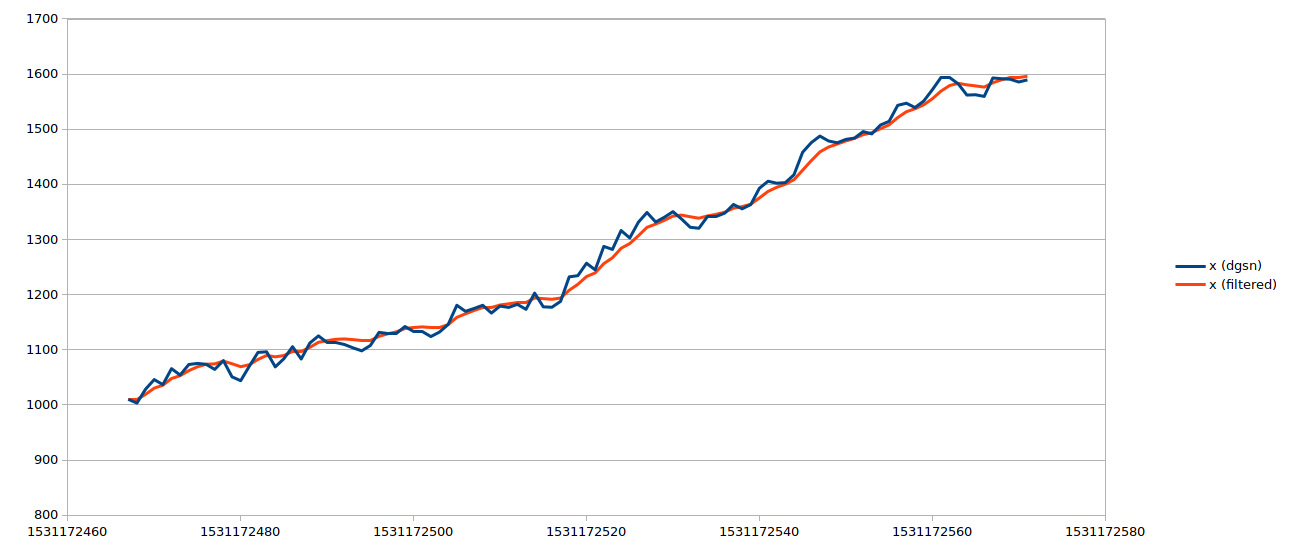
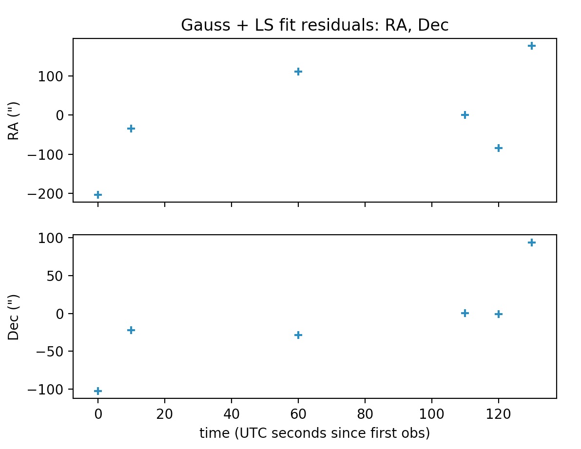
Similar to gauss_method_sat in call signature, but after applying the Gauss method to the subset of the observations defined by obs_arr, this function applies a least-squares procedure to the whole set of observations (unless otherwise selected by the user using the optional argument obs_arr_ls; see documentation), returning the Keplerian elements of the best-fit to the observations. Orbital elements are returned in kilometers, UTC seconds and degrees, and they are referred to the (equatorial) ICRF frame. More details may be found in the documentation and the examples.

Example output:

4.2 Sun-orbiting bodies: gauss_LS_mpc

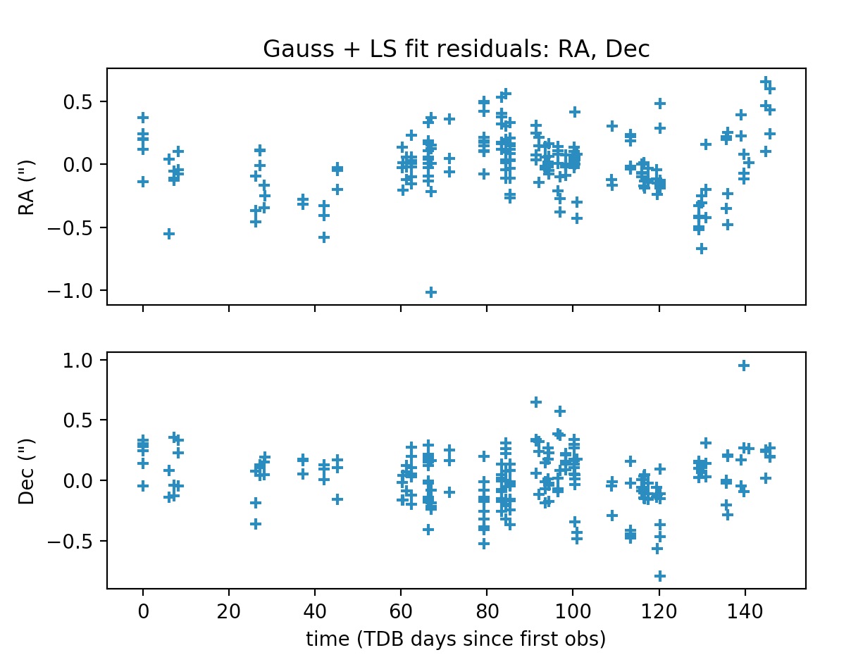
Similar to gauss_method_mpc in call signature, but after applying the Gauss method to the subset of the observations defined by obs_arr, this function applies a least-squares procedure to the whole set of observations (unless otherwise selected by the user using the optional argument obs_arr_ls; see documentation), returning the Keplerian elements of the best-fit to the observations. Orbital elements are returned in astronomical units, TDB days and degrees, and they are referred to the mean J2000.0 ecliptic heliocentric frame. More details may be found at the examples and the documentation.

Example output:

5. Acknowledgments and credits

We wish to thank the satobs.org community, who gave us valuable comments and suggestions, and also provided us with observations of the ISS and other civilian satellites. We also wish to thank the Mathematical Physics group at the University of Pisa, for all the helpful discussions and feedback which contributed to this work.

6. TODOs

  • Allow the user to select ephemerides from astropy: currently, the user is not allowed to specify the ephemerides to be used in the orbit determination of Sun-orbiting bodies.
  • Add perturbations: for Sun-orbiting bodies, add planetary and non-gravitational perturbations; for Earth-orbiting bodies, add oblateness and atmospheric drag to orbit model.
  • For IOD-formatted files, allow the use of other „angle subformats“. There are actually 7 ways to codify the angles in IOD format, but currently the code only allows the angle subformat 2. Subformat 2 was chosen because it is the most used in the Satobs community. Some of this subformats involve alt/az measurements, so in a future version the code should know how to handle alt/az measurements in addition to ra/dec measurements. This could be done, e.g., by using the (alt, az) -> (ra, dec) conversion functions from the astropy library.
  • Implement orbit determination algorithms for SDP/SGP4 models from ra/dec measurements.
  • Let the user choose between two possible values for the signed difference between two angles, instead of always choosing the shortest signed difference by default.
  • Add support for new or non-listed observatories in the MPC or the COSPAR lists of registered observatories.
  • Take into account the finite light propagation time, as well as atmospheric refraction.
  • Add support for radar delay/Doppler observations of Sun-orbiting bodies.
  • Add support for non-equal weights in least-squares subroutines.


[GSoC’18|Orbit-Determinator|Aakash] Implementing Two-Line Element (TLE) Input / Output and using it for evaluation

About the author: Hello everyone, I am Aakash Deep, I am a 4th year undergraduate student pursuing my degree in Bachelor's of Technology (B.Tech) in Computer Science and Engineering (CSE) from Indraprastha Institure of Information Technology, Delhi (IIIT-D) in India. I am a space enthusiast and I like travelling. My major hobby is speed-cubing.

About the organization

The organization for which I am working is AerospaceResearch.net. It has many interesting projects not only for the under-graduate beginners but for the masters‘ degree students too. We are a small group of enthusiasts who love to solve problems related to space. The benefit of being a part of a small group is that you get to know each other in a very short duration of time. We have regular meetings with our project mentors. The best part is that we can contact our mentors anytime. My mentor is Nilesh Chaturvedi who has guided me throughout the project and is still doing so. Alexandros Kazantzidis is also one of the mentors in the organization who cleared my doubts while building the propagation model.
Link to the organization repo.

Project

The title of the project is Implementing Two-Line Element (TLE) Input / Output and using it for evaluation.

What is TLE?

Two-Line Element (TLE) is a data format or a way of encoding various parameters of an object orbiting Earth at any particular time point, an epoch. TLEs can describe the trajectories only of Earth-orbiting objects. It is widely used as an input for projecting the future orbital tracks of space objects. A TLE set may include a title line preceding the element data, so each listing may take up three lines in the file. The title is not required, as each data line includes a unique object identifier code. The two lines contain a lot of information about the object and have a length of 69 characters each.

About Module

The scripts that were added to the module are database initialization, scraper, parser, Gibb’s method, and propagation model. More details about each element are as follows:

Database

Database contributes a major role in testing and generating the result of a module. In the beginning, we did not have TLE data. So, we decided that we will store TLEs from the celestrak website in the database. Now, it is time to choose which database we are going to use: SQL or NoSQL? Both the databases have their own advantages and disadvantages. After taking care of the needs and the data which we are going to store, we chose SQL based data. The reason behind this choice is that the input is well defined and structured. We only want to store 2 strings (that is, line 1 and line 2 of the TLE) at a particular time epoch. MySQL is used to store the data. The format of the data stored in the database is – timestamp, line 1 of TLE, line 2 of TLE. „[GSoC’18|Orbit-Determinator|Aakash] Implementing Two-Line Element (TLE) Input / Output and using it for evaluation“ weiterlesen

[GSoC’18|VisMa|Shantanu] Week #12-13: Packing Up

This is GSoC’18 log#06. Here I will cover on what I have done in week #12-13. Link to the previous log. The work in these two weeks involved packaging and documenting the code.

Done so far…

Deciding which packaging style to choose was a difficult task. Though there were a number of options available for packaging python apps I couldn’t find one which makes it simple for packaging it for windows. I managed to convert the source into a single executable file using pyinstaller but the performance was compromised.

„[GSoC’18|VisMa|Shantanu] Week #12-13: Packing Up“ weiterlesen

[GSoC2018|OrbitDeterminator|Arya] Orbit determination and propagation

Introduction

OrbitDeterminator is part of the bigger DGSN project by AerospaceResearch.Net. The Distributed Ground Station Network will be a network of thousands of ground stations across the globe. Together, these ground stations will track satellites cheaper and faster than conventional tracking stations. It will also get ordinary citizens involved in real space missions, so it is a win-win for everybody.

The purpose of OrbitDeterminator is to process the data coming from the DGSN and estimate the orbit of the satellite. It should also be able to predict the satellite’s location at any future time. This is the approximate workflow of the project:

(Note that the project is still under development so this workflow might change in future.)

My mentor was Alexandros Kazantzidis. He alongwith Nilesh Chaturvedi had worked on the preliminary orbit determination part last year. However the results could be improved. So I worked a little on that, but my main contribution was on real time tracking. As a side project I made a web application for one of the modules. I also cleaned the repo by adding a gitignore file and removing all temporary and IDE files.

Technical Details

The project is hosted on GitHub and made entirely in Python. It includes a requirements.txt and setup.py file. So it can be installed easily using pip. The project directory structure is quite simple and intuitive:

├── docs
└── orbitdeterminator
    ├── example_data
    ├── filters
    ├── kep_determination
    ├── propagation
    ├── test_deploy
    ├── tests
    └── util

Observation data is stored in the form of csv files in the following format:

# the data consists of 4 columns separated by spaces:
#
# time, x-coordinate, y-coordinate, z-coordinate
#
# for example:

1526927274 -5234.47464 4126.08971 -1266.52201
1526927284 -5272.8012 4094.65453 -1208.06841

Time is stored in unix timestamp format. Unit of distance (unless otherwise specified) is a kilometer. Keplerian orbital elements are stored in the form of a 1×6 numpy array:

kep[0] = semi-major axis
kep[1] = eccentricity
kep[2] = inclination
kep[3] = argument of perigee
kep[4] = right ascension of ascending node
kep[5] = true anomaly

Similarly, state vectors are stored in the form of a 1×6 numpy array:

s = [rx,ry,rz,vx,vy,vz]

This should be enough to get one started. For more help you can check the documentation.

Preliminary Orbit Determination (blog post)

Last year two methods of filtering were developed – the Savitzky-Golay filter and the Triple Moving Average filter. Two methods of orbit determination were also developed – the Lambert’s method and an interpolation method. However, they were not giving good results for certain kinds of data.

I made a new algorithm that fits an ellipse to the data, similar to fitting a line to a set of points. It gave better results than the previous algorithms so we decided to continue with it.

Propagation (blog post)

The real time tracking consists of two parts – propagation of state vector and the Kalman filter. For propagation we decided to use the SGP4 algorithm. It did the propagation excellently but was not stable with the Kalman filter. So I made a simple propagator. It uses numerical integration and takes into account atmospheric drag and the oblateness of the Earth. After making it I spent a lot of time testing it. The only major problem was that the time period did not match with the real time period. A simple fix for this was to manually fiddle with the semi-major axis of the satellite until it gives the correct time period. I tried a lot to fix this problem, but could not do so. Anyway, since it was working well with the Kalman filter, we decided to continue.

DGSN Simulator (blog post)

Since enough ground stations do not exist yet, we need some sort of artificial data to test the Kalman filter with. So I proposed to make a DGSN simulator module. The basic idea was that it will give the location of the satellite periodically with some noise. In the end the simulator had the following features:

  • Noise in spatial coordinates
  • Non-uniform interval between observations
  • Gaps in observations (to simulate the satellite being out of range)
  • Simulation speed control

The simulator in action. It is printing the coordinates every second.

Plotting the data produced by the simulator.

Kalman Filter (blog post)

After all this the Kalman filter was left. This was quite straight-forward. I directly implemented the equations on Wikipedia and it worked quite well. However if a time varying covariance matrix is used, it will give better results.

Web Application (blog post)

As a side project I made a web application for the ellipse fit algorithm. We created a new repository for this because it is not a necessary component of orbitdeterminator. It is made using the Dash library. Upload a csv file, it will process and give the orbital elements alongwith beautiful graphs.


The web application

List of scripts I created

Future Work

  • Integrating Aakash’s SGP4 module with the Kalman filter.
  • Fixing the time period problem in the numerical propagator.
  • Testing the system with real observations.
  • Improving the Kalman filter.
  • Deploying the web application on a public server.

Useful Links

[GSoC2018|USOC|Pedro] Final Evaluations – My 3 month stay at AerospaceResearch

After 3 months of work towards AerospaceResearch, the time has come to write my last devblog related to this year’s edition of GSoC.  This might be a long one, so please bear with me for the next few minutes. At the end of the post, there’s a section with all my work throughout the project.

Assigning data to UI elements

Since the last post, the AssignData Window has suffered considerable changes. I had to re-design it from scratch due to some limitations related to JavaFX’s TreeView implementation. Moving items from one tree to another causes them to behave incorrectly. I had to stick to another solution that may not look as smooth and intuitive but performs way better and actually works.


This is what it looks like:

„[GSoC2018|USOC|Pedro] Final Evaluations – My 3 month stay at AerospaceResearch“ weiterlesen

[GSoC2018|DirectDemod|Vinay] Week #9-10: Accurate Meteor M2 and Funcube Sync detection

In the last blog we discussed how we were able to get the constallation and thus the bits from the input file. In this blog we will look at how we are accurately obtaining the sync positions within the file.

„[GSoC2018|DirectDemod|Vinay] Week #9-10: Accurate Meteor M2 and Funcube Sync detection“ weiterlesen