During GSoC 2019, I worked on AerospaceResearch.net’s orbitdeterminator and orbitdeterminator-webapp project, the following is what I was able to add/test/modify to these exciting projects:
A custom perturbation module: Allows user to propagate orbital elements generated by gauss method in environments of different custom perturbations, incorporated SDP/SGP4 models and displays final co-ordinates and initial and final orbital elements.
Least square subroutines: Add support for non-equal weights in least-squares subroutines.
Conversion scripts: Added various functions helpful in orbit determination.
Parsing scripts and Inter-frame coordinate conversion, added support for all angle subformats in IOD data.
Field testing and validation with satobs community.
Comparison mode for web-app: Allows user to compare plots and results produced by various keplerian determination techniques.
Incorporated units, filters and keplerian determination techniques into the web-app.
Custom propagation module:
A script that allows the user to propagate keplerian elements generated by gauss method. Propagation module consists of environments for various natural and artificial perturbation accelerations. User can select ephemeris for sun orbiting bodies both while applying gauss method and while propagating. Options to select SGP4/SDP models for the propagation of earth orbiting satellites. User can change the values of various natural constants or use the default ones. Add option to use NASA NEO Webservice for (comets and asteroids) NEOs orbital data and add method for their propagation. Prints initial orbital elements and final (position, velocity) vectors and final orbital elements. Added support for all angle subformats in IOD format used by satobs.
More units, filters and keplerian determination techniques for web-app:
Added option to select Filters and Methods of Keplerian determination for determining the orbit.
User can now select from the following filters-
Savintzky Golay.
Triple moving average.
Both(Savintzky Golay and Triple moving average).
None (no filter).
User can now select the method of keplerian determination from the following-
Ellipse Fit.
Gibbs method.
Cubic Spline Interpolation.
Lamberts Kalman.
Comparison mode for web-app:
A script that allows the user to generate comparison plots for different filters/methods.
3-d animated plotting:
Better plots for simple visualization using matplotlib.
Conversion module:
Contains various conversion functions essential for further progress of this project.
2. Link to my GSoC 2019 project work:
The main part of the work I did is contained in the following modules:
Add support for radar delay/Doppler observations of Sun-orbiting bodies.
Add support for R.D.E. format data in orbit determinator.
Add support for all formats(IOD, RDE, UK) into the web-app.
Incorporate app.py and comparison_app.py into a single multi-page web-app.
Methods for coordinate conversion when slant range is not available.
Acknowledgment:
The success and final outcome of this project required a lot of guidance and assistance from my GSoC mentors(Arya, Aakash and Nilesh) and I am extremely privileged to have got this all along the completion of my project. All that I have done is only due to such supervision and assistance and I would not forget to thank them.
I owe my deep gratitude to Andreas Hornig(organization head), who took a keen interest in our project work and guided us all along. Also because of the system aerospaceresearch.net has developed over the years working for this organization gave me the freedom to expand my knowledge rather than just implementing stuff that I simply don’t understand.
We are almost in the deadline of GSoC, and I have been working in a project called MOLTO. I didn’t publish any blog until this moment since there has been a lot of work and I’ve been really busy. In this blog I will describe the whole process behind this project that has been changing since it begins.
It has been an amazing experience where I’ve learned a lot, I appreciate the time from my mentor David Morante who has been really involved during all the program. I would like to thank him for all the support. Thanks for giving me the opportunity of being part of this incredible program, all the knowledge I got from this is invaluable for me.
By the way, it’s time to talk about the project, it started with my application where they were asking for a student who could create or improve their user interface as well as do some improvements in the algorithm code. But before going away, I will explain in brief words what is MOLTO. At first, the application was for work in the MOLTO-IT project which is a branch of a bigger project called MOLTO. MOLTO is a mission designer created by David Morante for his doctoral thesis. He divided the project into three branches that I will describe below:
MOLTO-IT (Multi-Objective Low-Thrust Optimizer for Interplanetary Transfers): It is a fully automated Matlab tool for the preliminary design of low-thrust, multi-gravity assist trajectories.
MOLTO-OR(Multi-Objective Low-Thrust Optimizer for Orbit Raising): It is an application for the preliminary design of low-thrust transfer trajectories between Earth-centered orbits.
MOLTO-3BP (Multi-Objective Low-Thrust Optimizer for the Three Body Problem): is a fully automated Matlab tool for the preliminary design of low-thrust trajectories in the restricted three body problem.
My main proposal –was specifically for MOLTO-IT but at the end it changes– was about make a great UI without losing Matlab efficiency and without the need of re-build the code in another language. Since Matlab is very limited for UI purposes. I proposed to create an architecture that could enable the communication between Matlab and external applications, using their python engine through an API. That’s why my proposal is called MOLTO-IT As A Service (MaaS). I quote myself:
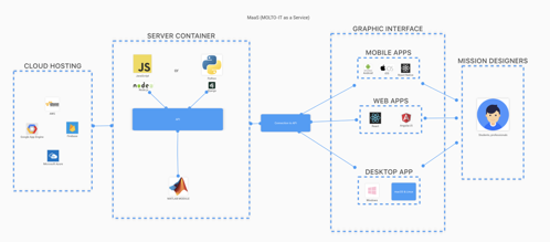
The objectives of this project are to find optimizations in MOLTO-IT trying to reach the best performance due to the hard numerical process that this project does and create an API using this Matlab module as a service where the users will send a POST request with the necessary inputs, and it will return the necessary information. Such as parameters of orbits, time, fuel consumed, or even graphs, etc. This will allow the team to create a better and more attractive graphical interface without losing the Matlab efficiency. Creating in this way, the possibility to use this service wherever you want such as mobile, web and desktop applications.
Image 1 – Architecture
Once we started talking about the project during the community bonding phase, we realized that we could improve the project thinking bigger and making some changes to the initial proposal. So we started thinking on work in MOLTO instead of only MOLTO-IT. Clearly, this new way to see the application changes some stuff such as primary design but the main goals will keep mostly the same.
Main Goals:
Extend capabilities of MOLTO-IT MOLTO.
Create API in selected programming language. (JS, Python)
If it is possible, create an MVP for MOLTO-IT MOLTO.
The proof of concept that I created for my application was some-kind different from how MOLTO looks right now. In the url below you can see my proof of concept of the API and UI during GSoC application:
And this one is the re-builded design after we started working on MOLTO. The flow was created in order to create a new mission in MOLTO-IT, so click start in MOLTO-IT button and just go through the flow:
As you can see there were some big changes, in my GSoC application I created a mobile application and I ended up creating a web application, but this iterative product development allow us to reach the main goal for MOLTO which was always to create an application available for anyone.
MOLTO IT
I will explain how MOLTO-IT works for avoid extra-explanations below, MOLTO-IT is the only one that right now is completely finished, MOLTO-OR and MOLTO-3BP are under development. We have been focused on making work this service, since OR and 3BP will work pretty the same.
MOLTO-IT is a fully automated Matlab tool for the preliminary design of low-thrust, multi-gravity assist trajectories. It means, it could allow us to know which is the best trajectory for interplanetary missions. Quoting its main goal:
The purpose of MOLTO-IT is to provide a fast and robust mission design environment that allows the user to quickly and inexpensively perform trade studies of various mission configurations and conduct low-fidelity analysis.
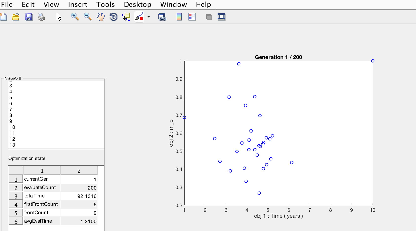
All of this is achieved through an outer loop that provides multi-objective optimization via a genetic algorithm (NSGA-II) with an inner loop that supplies gradient-based optimization (fmincon) of a shape-based low-thrust trajectory parameterization. At the end the mission designer will need to input a series of parameters, such as the spacecraft’s departure body, its final destination and some hardware characteristics (Launcher vehicle, mass, propulsion), as well as the range of launch dates, flight times and a list of available planets to flyby. The software tool then uses these data points to automatically compute the set of low-thrust trajectories, including the number, sequence and configuration of flybys that accomplish the mission most efficiently. Candidate trajectories are evaluated and compared in terms of total flight time and propellant mass consumed. This comparation is called pareto front and will look like this through the matlab plot:
Pareto front – matlab
After all the process is finished, we will be able to see the last generation which will contain the pareto points, every point is actually the best fit for the mission designer purpose, I mean if you want to go to mars and arrive in less than one year, you know that you will sacrifice most of your fuel, but if you are able to wait for a long travel such as 5 years, you will save up a lot of fuel. Whatever the point you select in the last generation, you could be confidence it is the most optimal solution. Btw, once you are in this part of the process you could select the most convenient pareto point for your mission and this will allow the tool to create the trajectory.
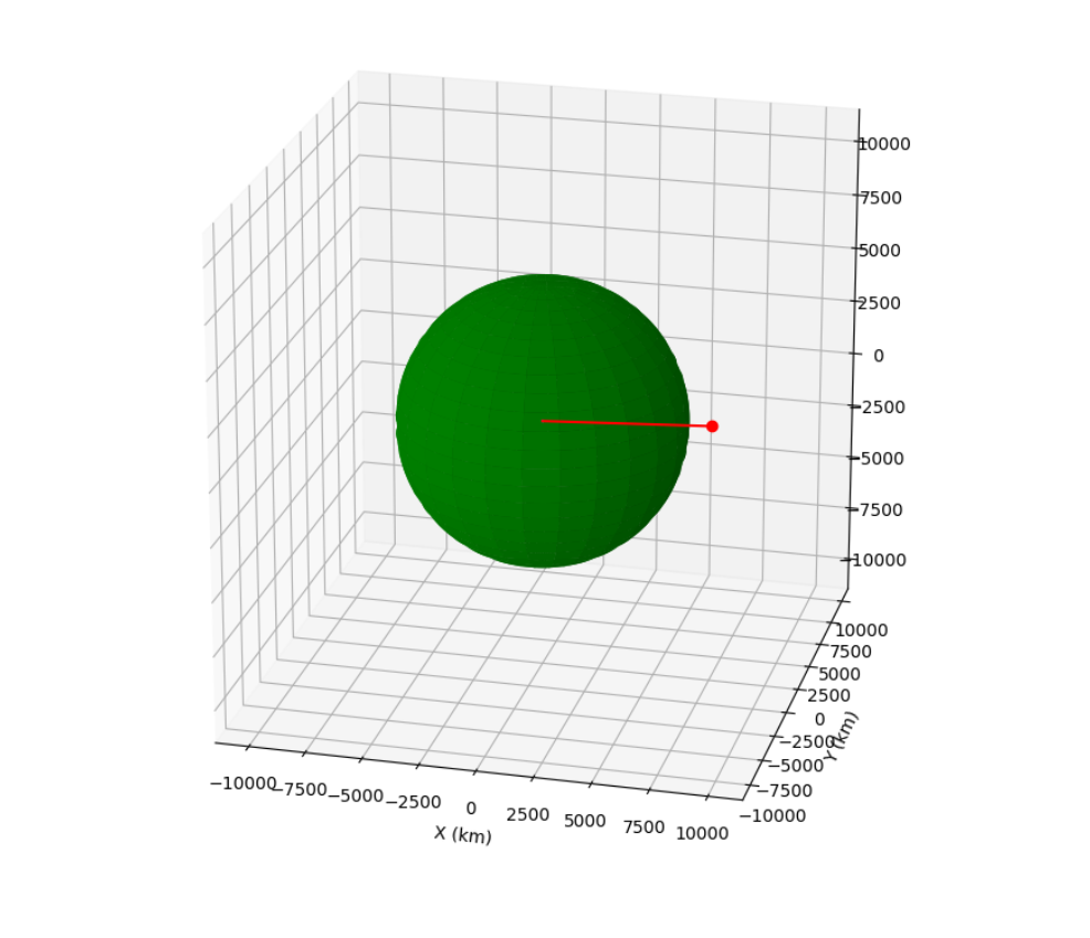
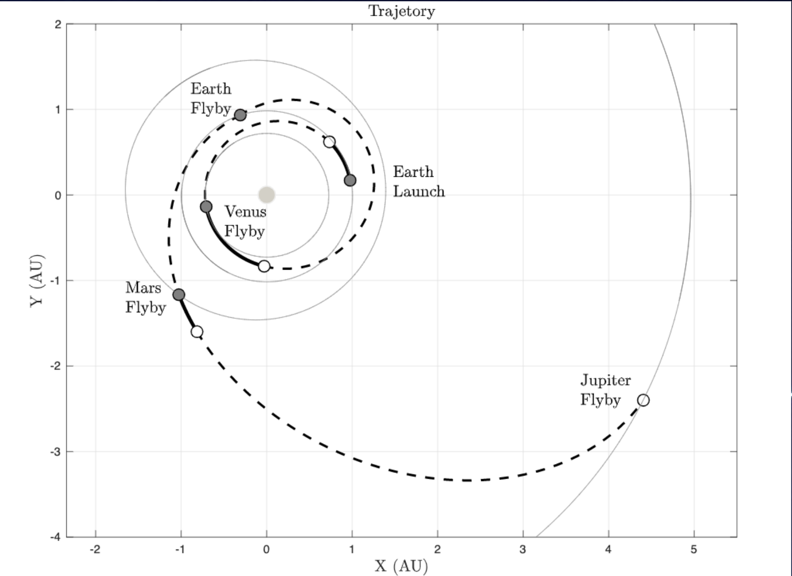
The trajectory is created by another functions that all they need is the mission configuration and the pareto point selected. After that you will be able to see the trajectory which will include everything a mission designer should know such as: Number of flybys, time, where to apply impulse, and more parameters, I attach an image below of how the plot looks like.
Dotted lines: No impulse Solid lines: Impulse
FIRST EVALUATION
All the process described before was during the phase of community bonding and maybe 1 week from first evaluation. During the first evaluation, I was mainly focused on the API since I need really double check everything will work. As you could imagine if something goes wrong with the communication between Matlab and the API, maybe anything could be possible.
The API was created within python language using flask, matlab engine for python, redis, celery, socket.io, and google drive (gspread). Why google drive? – It is something that I’ll talk about! –
The UI was created using React.js, Redux, socket.io client, recharts, and some other libraries. – Completely created using Hooks even for redux! –
During my regular meetings with David, we started thinking on what we’ll need to change in Matlab code in order to call the main function from the API. We quickly realized that we should change the main function in order to receive a json, at the end it was receiving an struct from an examples file. After that, a route was created in flask in order to receive the data from the UI, process it and finally send it to Matlab. The main purpose of using matlab python engine is that we could call Matlab functions within python, and the main function called „molto_it.m“ was the only one to call in order to trigger all the process. Until this point we were happy because everything was working like a charm. So I started working on the UI that finally looks some-kind different since I made some changes on-the-fly. We decided to implement an slider in the home page instead of the images, and implement a typer feature within the slider.
Dynamic component – Slider
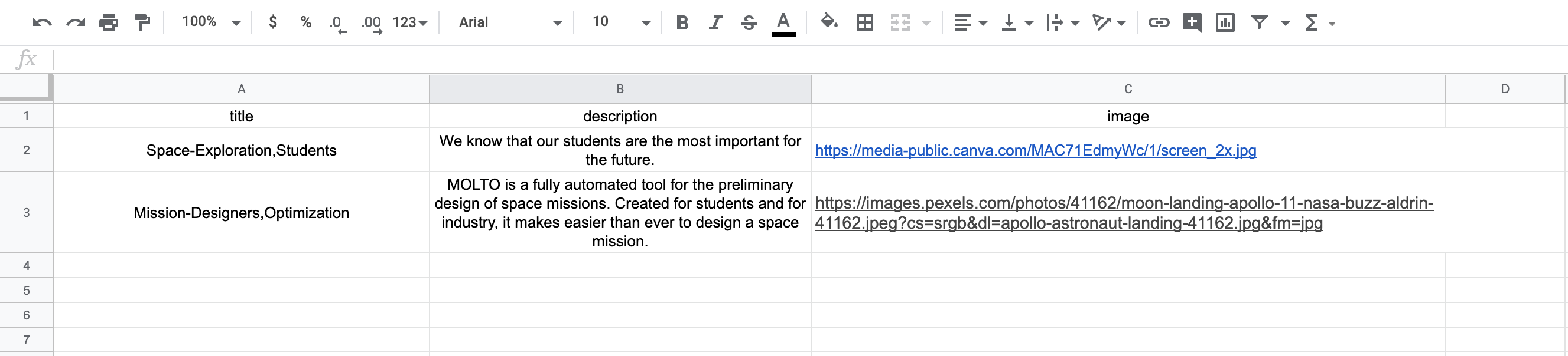
Excel file – Sliders
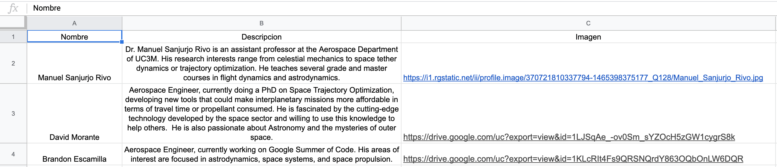
As we were advancing in the UI, we also realize that it would be a problem if all the content were static -We also think about the possibility to implement a user architecture to enable users save their missions, we knew that a database was needed but we were just trying to avoid it at least for GSoC purposes, but thinking in that feature for the near feature-. There is where Google Drive appears at least temporally, I proposed a feature where all the content could come from an spreadsheet that would be located in google drive, so every-time that we want to make a change, it would be as easier as just enter to the spreadsheet and change the content. Similarly for the collaboration component that would be updating the collaborators every so often. At the end, I would like to clarify that this feature will change, this was made just for MVP purposes. So, I finished my first evaluation implementing this feature that actually work effectively. ??
At this point, we needed to worry about the Matlab’s response since the process it’s composed by two main tasks: The pareto front and the trajectory. The real problem was that both of them plot the results, based on the real-time data. So one of our options were just to send an image of the final plot or just find a way to send the data in real-time trough the API to the frontend. But there was another problem, once the process start it was returning the generations in real-time, which was a problem because the API was making a POST request which will wait for one response, so in this way we were just able to receive the first generation.
We were having problems due to the synchronous naturalness of python. In this case, the requirement was to being constantly sending data to the UI, at least every-time the software creates a new generation, in order to display the data in real-time in the UI. –Such a task!- I thought in the feasibility of using sockets for the communication, but it was tricky because I would need a trigger to let me know once the generation is finished. And obviously all of this should be parallel to the request. Talking with David, we agreed that the best way was creating a new file every time the generation was completed, so in this way I could create a socket that should be constantly looking for files in a temporal directory. So that’s what we did, every user that creates a mission, creates a temporal UUID that will add a temporal directory within the server, so the Matlab function will redirect all the created files to this directory. Once you have the first generation you will be able to see in real-time the plot directly in the UI. All the directories will be deleted within the same day at night.
Waiting for files in the temporal directory.
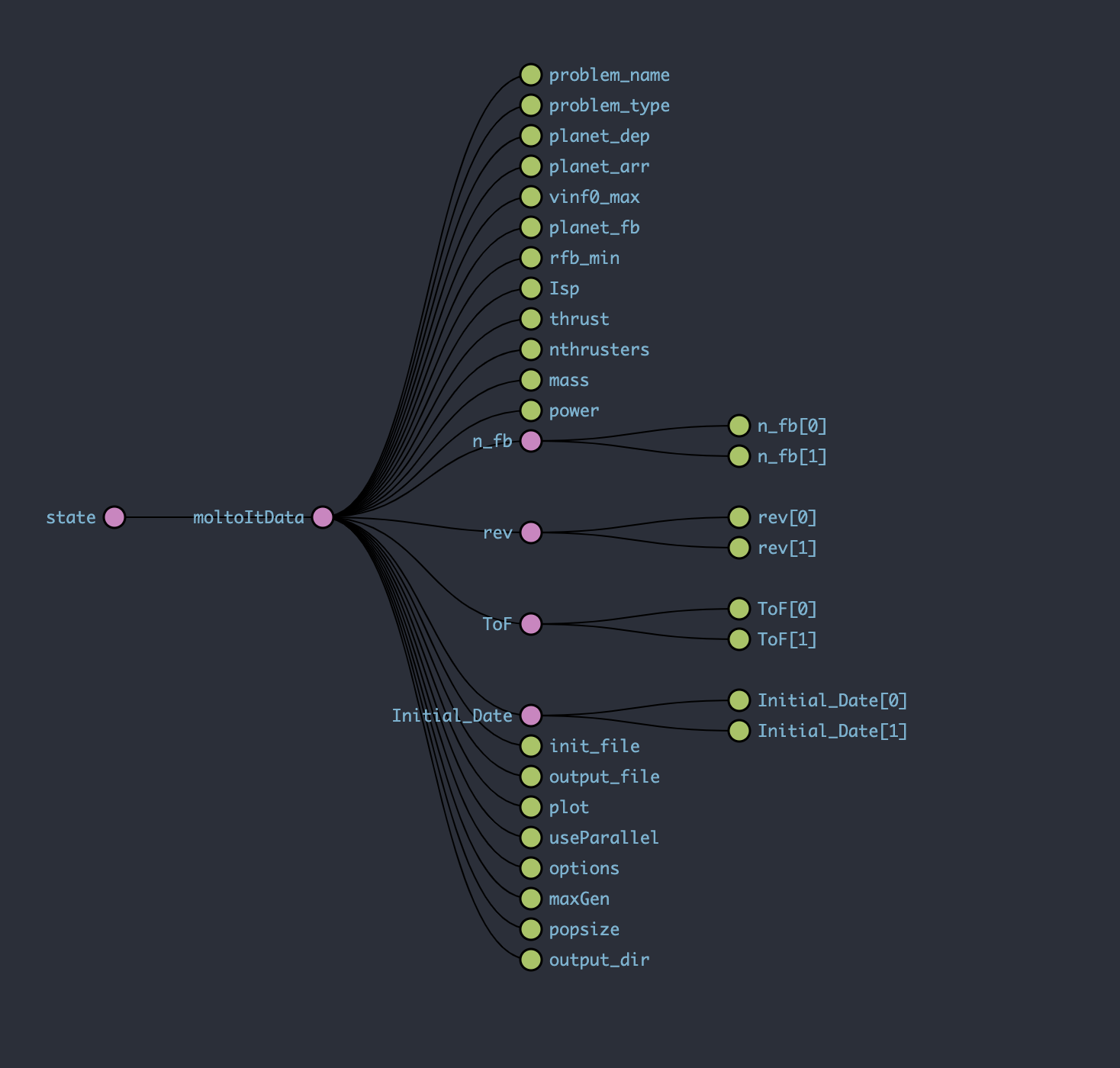
In that moment, we had almost all the first part to plot the pareto front, but in the UI we needed to catch all the data and save it in the correct way. We should be able to get the data in any moment, and this data should be available in almost the entire application. That’s why, I decided to use Redux. Redux is one of the best tools for data management if you using React, so I implemented the Redux architecture in order to handle all data from the API. At the end, the store looks like this.
Redux – Store
All the data come from a kind of form, where the user puts all the inputs in order to send the data to the API. This allows me to just send a POST request with all the data from the store, once the user finished all the flow, it also allows me to remember the selections of the user, so once you select something, you can go back and you will see that your selection is still there.
User flow – Form mission
FINAL EVALUATION
In the final evaluation we were trying to finish minor details such as design details. for example, we have been testing all the application using a dropdown where we need to select planets, but of course there should be a better way to do this. So, that was one of the big new features where I could work. So, I used a library to display the planets in a cool way. You already saw the planets feature in the gif’s that I put before, but I will leave here a static image of the feature.
Planets component
Of course, It was not all. In that point, we could plot the pareto front, but the last part requires to plot the trajectory, due to the times, we chose to just display the trajectory plot from Matlab in the UI, at least for GSoC purposes. ¿How we did it? As I explained before, once you get the final pareto front the user can select one point, the optimal point for your mission in terms of mass and time. So we call the API again at same route but this time with a flag. This flag means that you have the point of the pareto front that fits into your mission design, so Matlab function is enabled to detect it and just create the trajectory instead of call the genetic algorithm. Something cool is that you could go back and select another pareto point, and just call the API again. This will create the trajectory for the new selected point. It allows the users to iterate between different configurations for the same mission almost instantly. Btw, it finally looks like this – is the last view where you could share or download your preliminary results of your mission or create a new one.
Trajectory Plot
The last feature that I implemented is related to something we saw in the second evaluation. As you know python works synchronous and every task will be lineal. And also as you know until this point, every request will long as much as the number of generations the user request. So if the user request a genetic algorithm using 200 generations, the server will be busy a lot of time. The problem remains in the fact that if 3 users design a mission at the same time, they will probably have some issues because 2 of them will wait more than the normal request. So in order to avoid this issue, I started using threads, and parallel tasks. How I did it? Using celery, redis, and eventlet. This allow me to manage many requests and start them in the background. So the server is always available for new users without affecting the running times. ?
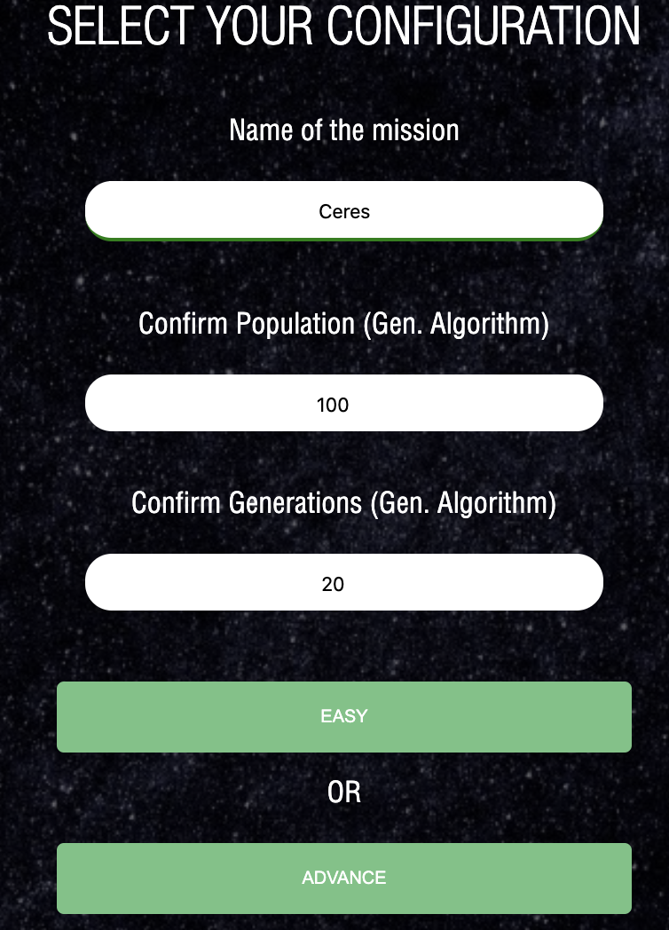
Initial Configuration MOLTO-IT – The only difference between easy or advance is how many configurations the user could edit. For GSoC purposes, we just worked in the easy one.
Celery is an asynchronous task queue/job queue based on distributed message passing. It is focused on real-time operation, but supports scheduling as well. The execution units, called tasks, are executed concurrently on a single or more worker servers using multiprocessing, Eventlet.
Eventlet is a concurrent networking library for Python that allows you to change how you run your code, not how you write it.
Redis is an open source (BSD licensed), in-memory data structure store, used as a database, cache and message broker.
Something cool that could be a new feature, is the fact that if the user remember the UUID that it creates within the mission. I mean if you could send it to the user through email, they could create the mission, go to take lunch or wathever, come back and put the UUID and the application will find the created directory, and will display the final plots in just seconds! —- This is possible thanks to the sockets we use to search for files and directories –
I would like to say that there are a lot of features that I didn’t take in count for this blog, just for become it short, since there is a lot of information. I just went through the most important features. But if you have some questions due to other component or something else. Please don’t hesitate in let me know. One last thing, the last month, we had some problems with the servers, that’s why there is no production application now, hopefully on monday 26 august, everything will work again, and then I will push the application to production. Once it works, I will edit this post in order to share it. Right now, everything is working under development.
What’s next?
As I wrote before, there are some TO-DO’s, where I will be working the rest of the year. We are open if anyone wants to contribute to this project.
1.- Create and implement architecture for save users and missions. (mongoDB)
2.- Send email with UUID, so the users could come back after they create the mission.
2.- CMS for sliders and collaborators.
3.- Improve responsive application.
Repositories:
You will find the documentation of every project within the readme.
ESDC (Evolutionary System Design Converger) is a software suite designed for optimization of complex engineering systems. ESDC uses system modelling equations, a database containing data points of existing systems, system scaling equations as well as mission requirements to design systems that fulfill their design objectives in the most efficient and effective way.
GSoC 2019 Contribution
The heart of ESDC’s optimization process is a genetic algorithm. The algorithm takes an initial population of design points and navigates the design space using a series of operations that are inspired from natural selection, such as mutation of permitted design degrees of freedom and subsequent selection, . One optimization cycle produces a lot of data and need to be analyzed and examined in order to acquire insight about the optimal designs, the performance of the algorithm and the design space in general.
My contribution to the project is a flexible multi-dimensional visualization and animation system designed for exploration of the system’s evolution data. The system uses various visual aspects of the generated visualizations in order to encode more degrees-of-freedom that would normally be possible in a simple 2-d or 3-d plot, thus allowing the exploration of complex systems. The definition of the visualizations is achieved through a user-defined XML file, where a plethora of options for customizing the content, the features and the annotation of the visualizations is available. The visualization system also has the ability to animate the generated figures, thus visually recreating the progress of the optimization.
Although the planned key features have all been implemented,
there is always room for improvement and as the ESDC project is growing additional
needs will arise. Currently, the main future work identified is:
-) Improved integration with ESDC, specifically automatically
acquiring names and units of the system’s degrees-of-freedom which can be used
in all annotations.
-) Automatic generation of additional data from data to
understand reasoning behind the final design. For example, presenting the
relevant data, where designed subsystems rely on.
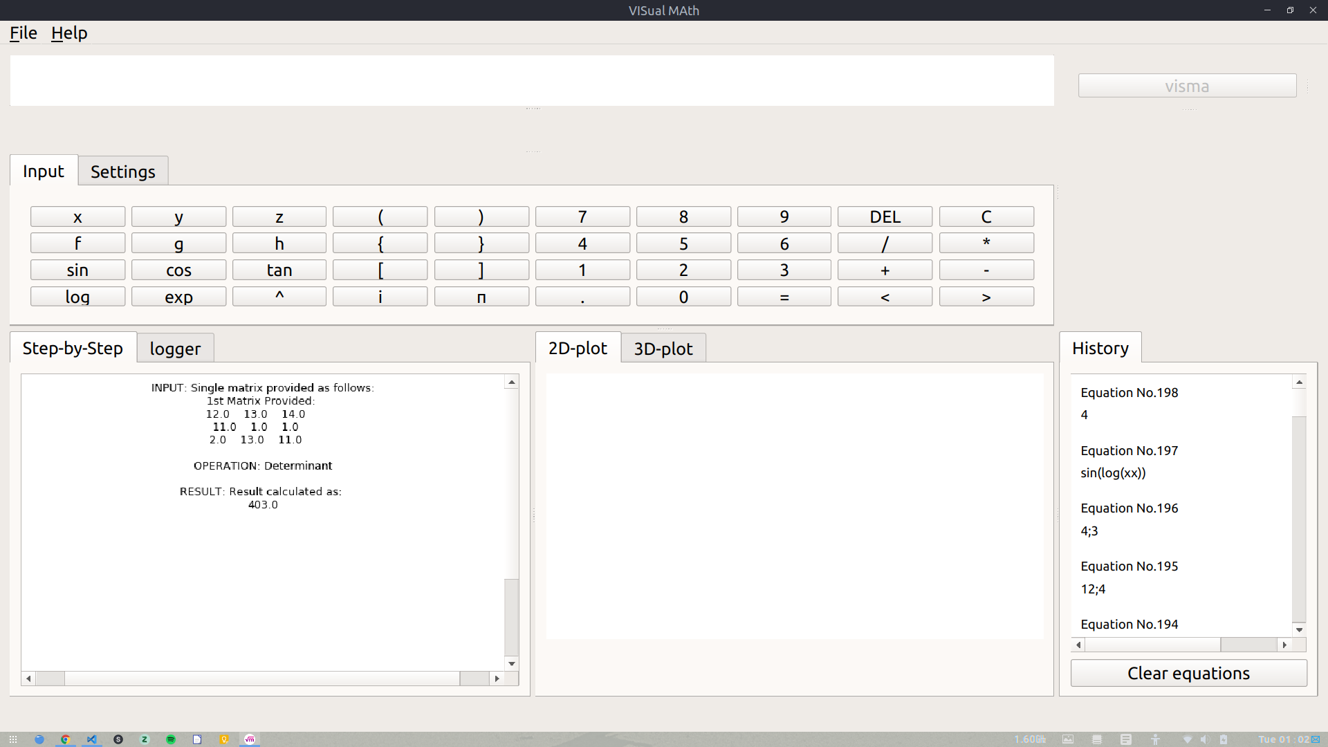
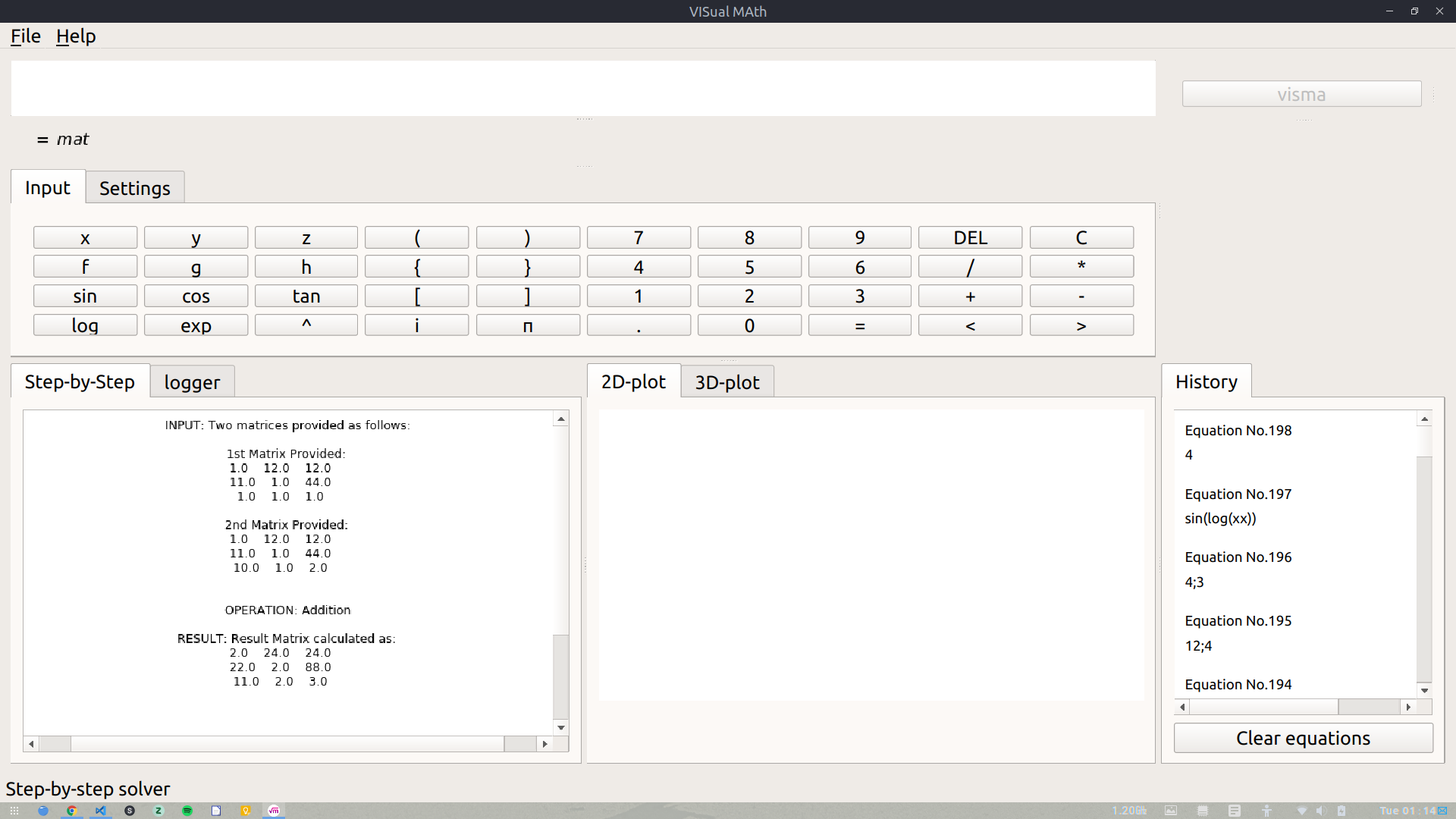
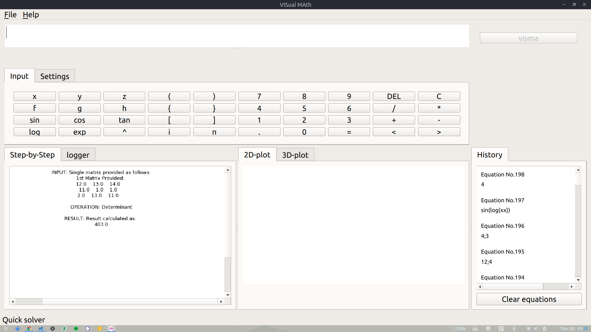
visma-VISualMAth, an equation solver and visualizer, which aims at showing the step-by-step solution & interactive plots of a given equation. As of now, VisMa is able to deal with matrices, multi-variable simultaneous equations & higher degree equations (up to four degrees) as well.
Via this blog, I will be giving a final wrap to everything I did during my wonderful stay at AerospaceResearch.net.
Before the start of GSoC 2019, following major deliverables were decided:
Re-writing simplify modules (addsub.py & muldiv.py) by using build-in class methods.
Adding support for Expression simplification
Adding a module for Discrete Mathematics
Adding support for equation solvers for cubic & biquadratic polynomials.
Adding support for simultaneous equations
Enhancing integration & derivation modules
Integrating matrix module with GUI
Rendering LaTex and Matplots in CLI
Including a Discrete Mathematics Module (including combinatorics, probability & statistics module)
All of the above-mentioned deliverables have been implemented. The commits referencing these changes are available at this link.
Below GIF shows the now integrated CLI module in action:
Some images showing matrix operations with VisMa are as follows:
Adding new modules & improving old ones was a great learning experience. Bugs were sometimes annoying however, each bug resulted in learning something new. That pretty much sums up all I did during GSoC.
I have written a developer blog for each of the Phases of GSoC, they are available as follows:
During the previous coding periods the key functionality
that was planned for this project was implemented. Thus, during the final
coding period there was time for improvements, development of one additional
feature whose inspiration came up during the previous period, refactoring and
organizing the file structure of the code as well as documenting the implemented
tool for feature users or developers.
First, the
following improvements were made:
-) The way
in which the minimum and maximum value of a continuous degree-of-freedom is
calculated was adjusted. Previously the minimum and maximum value was
calculated from the aggregate of the evolution data, which includes all lineages
and generations of the genetic optimization process. Now these values are
calculated specifically for each visualization scenario, only from the relevant
lineages and generations according to user defined options.
-) The part
of the code responsible for generating the animations was refactored and
extended to include the option to save the animations as compressed gif files.
The need for this arose after finding that the size of the gif files would
easily grow to tenths of megabytes even for the simple optimization scenarios
examined here.
Next, an
additional type of graphic, which allows for the visualization of useful
subsystems’ information on top of the existing 2d or 3d visuals was
implemented. This is a stacked bar graph spanning the y-axis on the 2d plots
and the z-axis on the 3d plots. The units of the stacked bar graphs are the
same as the units of the corresponding axis that it’s spanning. The height of
the individual bars of a stack are proportional to the values of the
corresponding degree-of-freedom of the respective subsystems that each bar is
representing.
Currently,
the stacked bar graphs are used to visualize the distribution of the electric
propulsion system’s total mass fraction into the corresponding subsystems.
Thus, the stacked bar graphs can be used to explore how the mass fraction of
each individual subsystem is changing as the genetic algorithms navigates
through different design points. To better understand this, let’s explore two
examples.
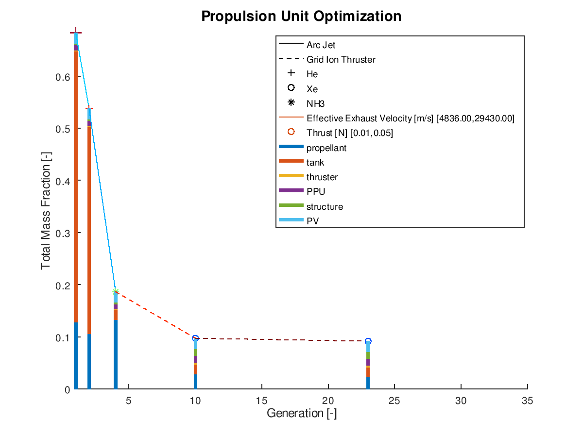
The first example is a 2d visualization, where the y-axis has been assigned to total mass fraction, the line style to propulsion system type, the line color to effective exhaust velocity, the marker to propellant and the marker color to thrust. Additionally, the stacked bar charts have been activated. As the y-axis corresponds to the total mass fraction, each bar of the stacks will correspond to the mass fraction of the respective subsystem. Only the best lineage is selected for visualization. The visualization system returns the following figure:
In the
figure above, we can examine how the mass fraction of each subsystem evolves as
the design of the system becomes optimal. In this simplified example, we can
see that the majority of the decrease of the total mass fraction can be
attributed to the reduction of the propellant and tank subsystems. Of course,
for this shrinkage to happen and the electric propulsion system to be able to
achieve the mission requirements, additional adjustments in other aspects of
the systems are being made by the optimization algorithm. Specifically, between
the starting and the final design point we can see that the propulsion system
type changes from Arcjet (solid line) to Grid Ion Thruster (dashed line), the
propellant changes from He (crosshair marker) to Xe (circle marker), the
effective exhaust velocity is increased (line color turns deep red from light
blue and “jet” is the chosen colormap) and the thrust is decreased (marker
color turns deep blue from deep red and “jet” is the chosen colormap).
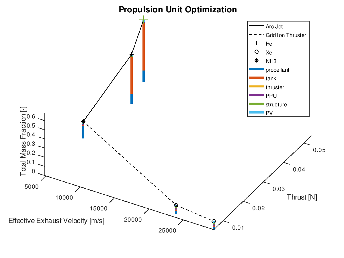
The stacked bar graphs can also be activated in 3d visualizations. In this next example, the x-axis has been assigned to effective exhaust velocity, the y-axis to thrust, the z-axis to total mass fraction, the line style to propulsion system type and the marker type to propellant. Only the best lineage is selected for visualization. The visualization system returns the following figure:
Like the
previous example, it’s easy to point out that the reduction of the total mass
fraction can be greatly attributed to the reduction of the propellant and tank
subsystems.
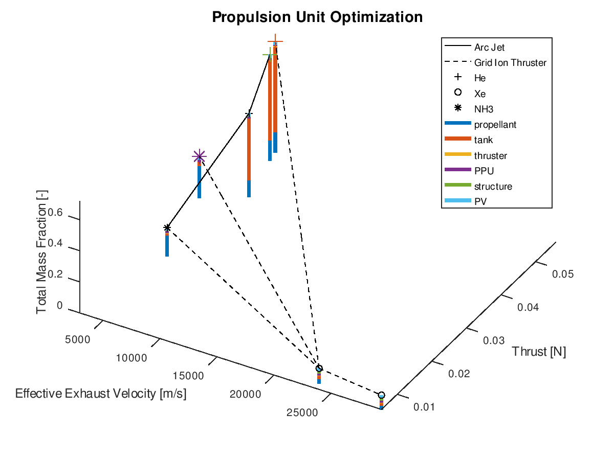
When using the stacked bar graphs in the 3d plot, it is also practical to include more lineages in the visualization. Selecting the three best lineages, the visualization system returns the following figure:
After this
final feature was implemented, additional refactoring of the code was done to
simplify certain parts and achieve improved extendibility and readability.
Refactoring the code was also done to end up in a restructured organization of
functions into subfolders. As the visualization system was designed with
flexibility, modularity and extendibility in mind, it is consisted of more than
100 functions. For this reason, a function dependency graph proved a great aid
for understanding the existing dependencies and making the appropriate
refactoring and restructuring decisions.
Finally, additional
documentation was created for this project to accompany the blog posts during
GSoC. All details regarding the available options and settings for configuring
the visualization system according to specific needs can be found in the
documentation. There, one can also find ready to use XML input file templates
which correspond to the visualizations found in all GSoC blog posts.
Congratulations
if you ‘ve made so far, this was the last long post! A final report will also
be released very soon!
This Project for this year’s edition of Google Summer of Code was titled: Decoding of ADS-B(Automatic dependent surveillance—broadcast)and Multi-lateralPositioning.
The aim of the project is to decode ADS-B frames/messages from raw IQ streams recorded using RTL-SDR radios and extract the data from these frames such as aircraft identifications, position, velocity, altitude etc.
The next part is to find the location of an aircraft when it sends a frame not having any position data in it’s payload using multilateration.
What is Multilateration ?
Multilateration is a method by which the location of an aircraft (can be any moving object which broadcasts a signal) using multiple ground stations and the Time Difference of Arrival(TDOA) of a signal to each ground station.
Implementations
Identification of long(112 bit) and short(56 bit) frames.
With the long frames, identifying each type of frame and the data contained in it.
Decoding and extracting the available data in the payload according to the frame type.
Building and outputting JSON files containing ADS-B frames and decoded data. (Gzipped)
Loading of files from multiple stations simultaneously.
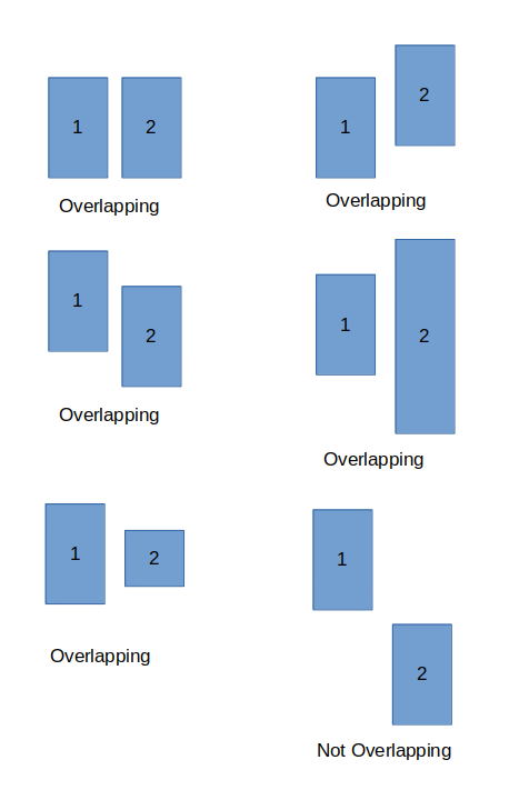
Checking and grouping files which were recorded during the same time or have overlapping recording intervals.
Searching unique signals/frames in the overlapping files across different stations.
Testing
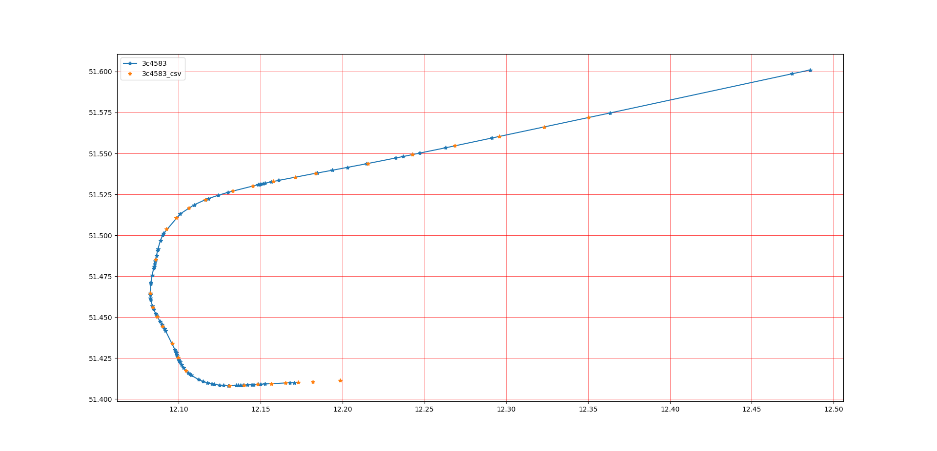
Since, position is one of the key component to this project, the first phase of testing was aimed at finding any hidden logical bugs in the code which calculates the position from the position containing frames.
As mentioned in the previous blogs, two methods are used to calculate the location.
The result obtained:
The plots in ‚yellow‘ are obtained from 3rd party trusted sources. This is a comparison plot of ‚our‘ output with trusted sources.
The project is expected to process files from several stations (5 stations) together. Thus there was a requirement to find files from different ground stations which were recorded at the same time interval. It can also be that the a part of the file overlaps. After which the ‚unique‘ frames were searched in these files.
The file overlap checker was tested with recordings from 5 stations recorded on 16th February in Germany.
This test run could find ‚unique‘ frames which were occuring atmost thrice, present at different ground stations.
Foremost, I would like to extend my sincere gratitude to my mentor and organisation head Andreas Hornig, for mentoring me throughout the season. Since I am not pursing a major in Computer Science altough coding and so called ‚cool stuffs‘ is my second hobby and passion, I would also like to appreaciate the additional energy and effort he has put in guiding me.
Besides, I put forth my vote of thanks to the organisation (Aerospaceresearch.net) as a whole, all the other mentors and the fellow students for making this organisation what it is and providing me with the opportunity to work on an open-source project.
In this blog post, I will be summarising all the work done during phase III (i.e. last phase of GSoC 2019).
This phase the major target was to wrap up all the work done during Phase I and Phase II. The first target was to implement GUI & CLI in matrices. The integration of GUI & CLI in matrices was pending from a long time and this was the time to get it done. The integration, however, was a bit tricky as it was very obvious that the usual parsers and tokenizers could not be used to integrate Matrices with GUI/CLI. We had to make an entirely new module which would be able to parse matrices (i.e. accept them as some input from the user and perform operations accordingly on them). We finally were able to properly integrate this module in GUI/CLI. It was worth the time & patience as the results were good. For now, the user has to enter the matrices in some specific Python list type pattern. In later versions, we can add options for adding matrices interactively by GUI.
Some screenshots of Matrix Module in action are:
The next part was adding test cases for Statistics modules (which were implemented during Phase II). Also, we added Equation Plotting feature in CLI during this part. It involved creating another Qt window equivalent to the plotter used in GUI version.
The last target of this phase was to add code to deal with cases when the Constant was raised to some fractional or Expression power. Earlier VisMa was able to handle only those cases when power was some Integer. The solution to this problem was to consider all the exponents as some object of Expression Class. Now since Expression simplification was done earlier this could be achieved. Also, I added the cases when Expression classes are involved in the Equation inputted by the user. Finally, our last target was to add the necessary documentation so that new users can get comfortable with the codebase. Personally, when I started to contribute to the project I found a lot of help because of docstrings & comments. Earlier developers (My mentors) have maintained a very well documented codebase, so it was my responsibility to carry this tradition forward.
To sum up, all the work done I am updating a list of all that we achieved during GSoC. The Changelog is as follows:
1. Simplify module written in Object-Oriented Programming Design.
2.__add__, __sub__ ,__mul__ & __truediv__ methods for most of the classes (like Constant, Expression, Trigonometric etc) have been added.
3. Discrete Mathematics Module has been added: a. Combinatorics modules like Combinations, Permutations & Factorial modules (with GUI/CLI implementations) b. Statistics Module containing mean, median and mode c. Simple probability modules d. Bit-wise Boolean Algebra module
4. Simultaneous Equation solver has been implemented
5. The plotter is now able to plot in both 2D and 3D for equations having one, two or three variables. It has been implemented in the CLI version
6. Equation solvers for higher degrees (Third & fourth degree) using determinant based approach have been added.
7. Integrations and differentiation modules are now implemented in all Function Classes (Trigonometry, Exponential and Logarithmic)
8. Integration & Differentiation modules have been rewritten to follow Object-Oriented Style.
9. Product Rule for Differentiation & Integration by parts module has been added.
10. Tokenize module is now improved to consider power operator (earlier it ignored power operator in many cases)
11. With above improvement Expressions raised to some power are duly handled by VisMa.
12. Parsing modules for printing matrices in Latex and string form have been added. With this matrix operations are now well implemented in GUI & CLI.
13. Expression simplification is now completely supported by VisMa. Almost all cases of Expression classes being involved in input equation have been taken care of. Multiple brackets are now also taken care by VisMa (for this the modules using recursion have been implemented).
14. The cases where Constant are raised to some fractional power or some solvable term have been covered.
The points where we will be working now are:
1. We can implement an Equation Scanner in the project. This way a user will be able to scan an image of the equation and it will be solved by VisMa. This was an idea during this GSoC but due to time constraints, we were not able to work in it for now.
2. VisMa is not friendly with Trigonometric expressions, there is a need to deploy some code in simplification module for taking care of this thing.
Overall, working in this community as a GSoC student was a great experience. It was hard but fun to stay within deadlines, fixing bugs, deploying new ideas etc. Feel free to connect with me on Twitter (https://twitter.com/mayank1Dhiman) & GitHub (https://github.com/mayankDhiman).
I discussed about how I am decoding the position of the aircraft from 2 ADS-B frames and also from 1 ADS-B frame and a reference position and how I found both handsome and erractic readings.
Let’s look into how other airborne parameters, such as ‚aircraft identity‘ and ‚velocity‘ are being decoded and calculated.
There is a special type of frame which is known as ‚Enhanced Mode-S‘ frames. They also contain similar information at times like the non-Enhanced Mode-S frames. I will elaborate on both in this blog.
Frames with downlink format 20 & 21 are known as Enhanced Mode-S frames.
The following methods were implemented in the code for decoding the information from the ADS-B frames.
Aircraft Identification
Frames with Downlink Format 17-18 and Type Code 1-4 are known as aircraft identification messages.
The structure of the 56-bit DATA field of any such aircraft identification frame will be as follows:
TC
EC
C1
C2
C3
C4
C5
C6
C7
C8
5
3
6
6
6
6
6
6
6
6
TC: Type Code
EC: Emitter Code
Second row signifies the bit-length
The EC value with regard to the TC value determines the type of aircraft (Such as : Super, Heavy, light etc). When the EC is set to ‚zero‘ signifies such information is not being transmitted by the aircraft.
An Airbus A380 is known as 'Super' and a Boeing 777-300ER is known as 'Heavy'. Small, private or training aircrafts such as Cessna 172s are known as 'Light'.
For determining the callsign a lookup table is used:
‚#‘ signifies a null value and ‚_‘ signifies a space between two words.
Let us take an Aircraft identifier frame recorded by one of our ground stations:
a0001910200490f1df2820700716
Thus the DATA part of this frame is:
200490f1df2820
BIN
00100000
000001
001001
000011
110001
110111
110010
100000
100000
INT
4
1
9
3
49
55
50
32
32
CHAR
[TYPE CODE]
A
I
C
1
7
2
_
_
The integer number corresponds to the corresponding element in the lookup table array.
Thus, the decoded callsign is „AIC172“ which belongs to Air India on the route 172
BDS 2,0 frames are also known as Aircraft Identification Messages. In these frames the first 8 bit of the DATA segment contains the BDS number and the rest is same as the previous one.
Airborne Velocity
ADS-B frames with Downlink Format 17-18 and TC 19 contain the velocity information of the aircraft.
Subtype 1 (Ground Speed)
The typical structure of the frame:
Position in frame
Position in data block
Length
Abbreviation
Data
33 – 37
1 – 5
5
TC
Type code
38 – 40
6 – 8
3
ST
Subtype
41
9
1
IC
Intent flag
42
10
1
RESV_A
Reserved-A
43 – 45
11 – 13
3
NAC
Velocity uncertainty (NAC)
46
14
1
S_ew
East-West velocity sign
47 – 56
15 – 24 change
10
V_ew
East-West velocity
57
25
1
S_ns
North-South velocity sign
58 – 67
26 – 35
10
V_ns
North-South velocity
68
36
1
VrSrc
Vertical rate source
69
37
1
S_vr
Vertical rate sign
70 – 78
38 – 46
9
Vr
Vertical rate
79 – 80
47 – 48
2
RESV_B
Reserved-B
81
49
1
S_Dif
Diff from baro alt, sign
82 – 88
50 – 56
7
Dif
Diff from baro alt
These two bits determine the direction at which the aircraft was flying:
S_ns:
     1 -> flying North to South
     0 -> flying South to North
 S_ew:
     1 -> flying East to West
     0 -> flying West to East
The speed and the heading can thus be computed by:
If the calculated heading is negative, then we add 360 to it.
Vertical Speed
The S_Vr bit (69) determines the direction(ascent/descent).
0- Up
1- Down
Therefore the actual speed is calculated by:
V = (int(Vr) – 1) * 64
Therefore, V is the speed and S_Vr states whether the aircraft is climbing or descending.
The VrSrc field (Vertical Rate Source) determines the measured altitude type:
Here let us see how the structure of Subtype 3 differs from Subtype1:
Position in frame
Position in data block
Length
Abbreviation
Data
33 – 37
1 – 5
5
TC
Type code
38 – 40
6 – 8
3
ST
Subtype
41
9
1
IC
Intent change flag
42
10
1
RESV_A
Reserved-A
43 – 45
11 – 13
3
NAC
Velocity uncertainty (NAC)
46
14
1
S_hdg
Heading status
47 – 56
15 – 24
10
Hdg
Heading (proportion)
57
25
1
AS-t
Airspeed Type
58 – 67
26 – 35
10
AS
Airspeed
68
36
1
VrSrc
Vertical rate source
69
37
1
S_vr
Vertical rate sign
70 – 78
38 – 46
9
Vr
Vertical rate
79 – 80
47 – 48
2
RESV_B
Reserved-B
81
49
1
S_Dif
Difference from baro alt, sign
82 – 88
50 – 66
7
Dif
Difference from baro alt
Heading
The S_hdg bit shows whether heading data is available or not:
0 - Heading data not available
1 - Heading data available
If heading data is available then it is calculated by:
Heading = Hdg(10 bit data) * 360/1024
Velocity (Airspeed)
Simply converting the AS bits gives the airspeed in knots.
Vertical Rate is calculated in the same manner as in Subtype 1
Enhanced Mode-S:
Aircraft Intention (BDS4,0)
The structure:
Field
Position
Length
Status
1
1
MCP selected altitude Precision = 16ft
2-13
12
Status
14
1
FMS selected altitude Precision = 16ft
15-26
12
Status
27
1
Barometric setting (in mb and not hPa) Value is actual minus 800 Precision = 0.1mb
28-39
12
Reserved
40-47
8
Status
48
1
VNAV hold state
49
1
ALT hold state
50
1
APP hold state
51
1
Reserved
52-53
2
Status
54
1
Altitude source: 00: Unknown 01:Aircraft altitude 10: MCP set altitude 11: FMS set altitude9
55-56
2
Note: MCP stands for Mode Control Panel where the pilot feeds in the data to the autopilot
FMS stands for Flight Management Computer where the data is fed to calculate various other flight parameters.
Track and Turn (BDS 5,0):
Many more information is given such as roll angle, true track angle etc:
Field
Position
Length
Status
1
1
Sign, 1
1
1
Roll angle range = [-90, 90] degrees Precision = 45/256 degree
3-11
9
Status
12
1
Sign
13
1
True Track angle Precision: 90/512 degree-
14-23
10
Status
24
1
Ground Speed Precision: 2 knots
25-34
10
Status
24
1
Sign
36
1
Track angle rate Precision: 8/256 degree/second
37-45
8
Status
46
1
True Airspeed Precision: 2 knots
47-56
10
Note: The sign bit determines whether to use 2's complement to determine the value present after it. It it is set to '1' then we have to use 2's complement.
Airspeed and Heading (BDS 6,0)
A lot more information is conveyed in this kind of frames:
Unfortunately the percentage of decodable Enhanced Mode-S message received was very low in both short recordings and long recordings which was worth hours.
File overlap checker:
The ground stations were programed to span each recorded file for 2 minutes(approx.). Now this means that for a long duration, there will be an array of files from several ground stations.
There has to be a logic, where the code finds all the files from several ground stations recorded at the same or has overlapping recording times and club them together for the next step.
I identified few such cases of overlaps:
The overlapping files are clubbed together into a list for further processing.
Next step is to find the same frames present in different station recordings, so we need to know the files that overlap and process it accordingly.
In this blog, I will summarize all the work, that has been done during my three months of work at AerospaceResearch.net.
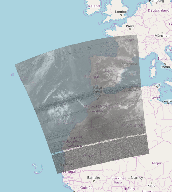
The resulting product is a fully functional web application and a set of supporting logic, that allows uploading, georeferencing, combining and displaying NOAA weather images. Below, more specific features are listed.
Work done
implemented functionality to extract and store satellite metadata
designed and implemented an accurate image georeferencing algorithm
designed and implemented an algorithm to merge several satellite images, taking care of overlapping areas
created CLI interfaces for each part of package API
implemented generation of web map and virtual globe
built custom web application, which includes web server backend with Flask and frontend
deployed the working application to the web (demo version at http://206.81.21.147:5000/map)
wrote tests, documentation, installation instructions and usage tutorials
For installation please see the installation guide in the repository description. To start using specific features please refer to the tutorials page, it contains usage examples with corresponding sample files for each use case. If you want to know more about how the software is working, please read my blogs. They describe in sufficient detail how the software is working.
Further work
Set up automatic data uploading from recording stations.
Set up a DNS domain.
Support
If you have any questions or issues concerning the usage of the software you can ask for help / open issues on GitHub or contact me directly.
This blog post will describe in general terms the architecture of web application, main steps of deployment process, processing server and several additional features.
General App Architecture
The application is an end-to-end data processing pipeline starting from raw satellite signal recordings and ending with displaying of combined images on the map or virtual globe. The image below describes this in a more structured way.
Figure 1. App architecture.
As showed on the image, the app consists of 4 main parts:
Recording stations
Processing server
Web server
Frontend
Data is being passed along this processing chain. Functionality of each part will be described in following parts of the article.
Processing Server
The task of processing server is to gather the raw satellite signal recordings and transform it to georeferenced images. This transformation happens using directdemod API:
DirectDemod decoder extracts the image from recording.
Image is preprocessed, two channels are extracted.
Each part is georeferenced and saved.
Processed data is being sent to web server.
Server uses ssh connection to securely transmit data, namely scp command is used. SCP stands for Secure Copy, it allows secure transmission of arbitrary files from local computer to remote machine.
Web Application
Web application is implemented using Flask. Web server has the following structure:
Figure 2. Web server.
It contains two main directories images/ – stores uploaded georeferenced image and tms/ – stores Tile Map Service representation of processed images. Images could be uploaded in two ways, either via ssh or throught /upload page (could be removed in production for safety reasons). After upload is done and the images are properly stored, then server will automatically merge this images using directdemod.merge and create TMS, which will be saved in tms/ directory. After processing is done, metadata will be updated and images will be displayed on website. Website itself contains 3 pages:
map.html
globe.html
upload.html (may be removed)
Map page displays images on Leaflet webmap, globe page uses WebGLEarth library to display images on Virtual Globe.
Should be noted that final implementation is somewhat different then showed on figure 2. Ability of viewing different channels was added, therefore tms stored in 2 directories corresponding to each channel.
Figure 3. Image of second channel.
Another major feature is called „Scroll in time“. Images are stored in chronological order and could be viewed sequentially using special slider. For each entry both channels could be viewed using a toggle button.
Deployment
Application has been deployed to the web http://206.81.21.147:5000/map. Appropriate domain name will be set up shortly.
Conclusion
This is the final part of the GSoC project. All main functionality and features have been implemented, web application is up and running.