[GSoC’21|Calibrate-SDR|Ayush] DVB-T for calibration

Hi everyone. I am writing this blog to share my work progress with everyone out there.

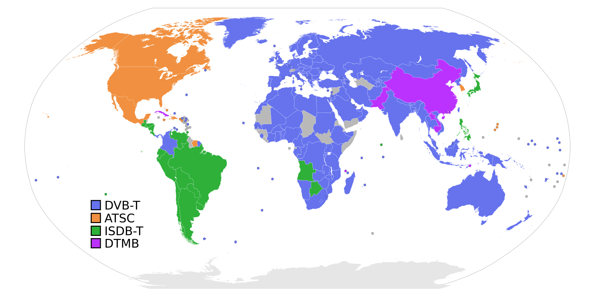
I have been working on extending the limitations in the Calibrate-SDR tool by adding support of DVB-T and DVB-T2 (terrestrial) signals. Because these signals are broadly used in Europe, Africa, Australia, and Asia region. So can be used here to provide calibration to more SDR users.

Visit here – http://www.dtvstatus.net/map/map.html

So the question arises What exactly I’m I doing?

As many of you would have worked on some sort of SDRs, might have faced errors due to the Frequency Offset of the Device(due to Crystal oscillators heating).

So here we have a tool named Calibrate-SDR to save you from correcting frequency offset repetitively. Calibrate -SDR is based on the idea of synchronization of devices by a constant frequency part present in the signal. This tool currently uses DAB+ signals to calculate the PPM shifting in frequency. I am enhancing it by using the DVB-T signal for this purpose and try to help more people out there.

Further reading about initial Calibrate-SDR refer to this blog.

Some words of wisdom about DVB-T signal

DVB-T, short for Digital Video Broadcasting — Terrestrial, is the DVB European-based consortium standard for the broadcast transmission of digital terrestrial television that was first published in 1997[1] and first broadcast in Singapore in February 1998. This system transmits compressed digital audio, digital video, and other data in a MPEG transport stream, using coded orthogonal frequency-division multiplexing (COFDM or OFDM) modulation. It is also the format widely used worldwide (including North America) for Electronic News Gathering for transmission of video and audio from a mobile newsgathering vehicle to a central receive point.

Wikipedia

Thanks to Wikipedia for providing historical details about this signal.

Some Technical Details about signal.

Would suggest reading the technical standard for more detailed idea about it.

https://www.etsi.org/deliver/etsi_en/300700_300799/300744/01.06.02_60/en_300744v010602p.pdf

I would cover only the part that was of value for me. Going through this paper and some research. I found out that DVB-T signals have a constant part called pilot inside the ODFM frame structure of DVB-T.

Visit etsi.org for better image.

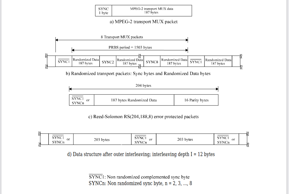
So in addition to the transmitted data an OFDM frame contains:

– scattered pilot cells;

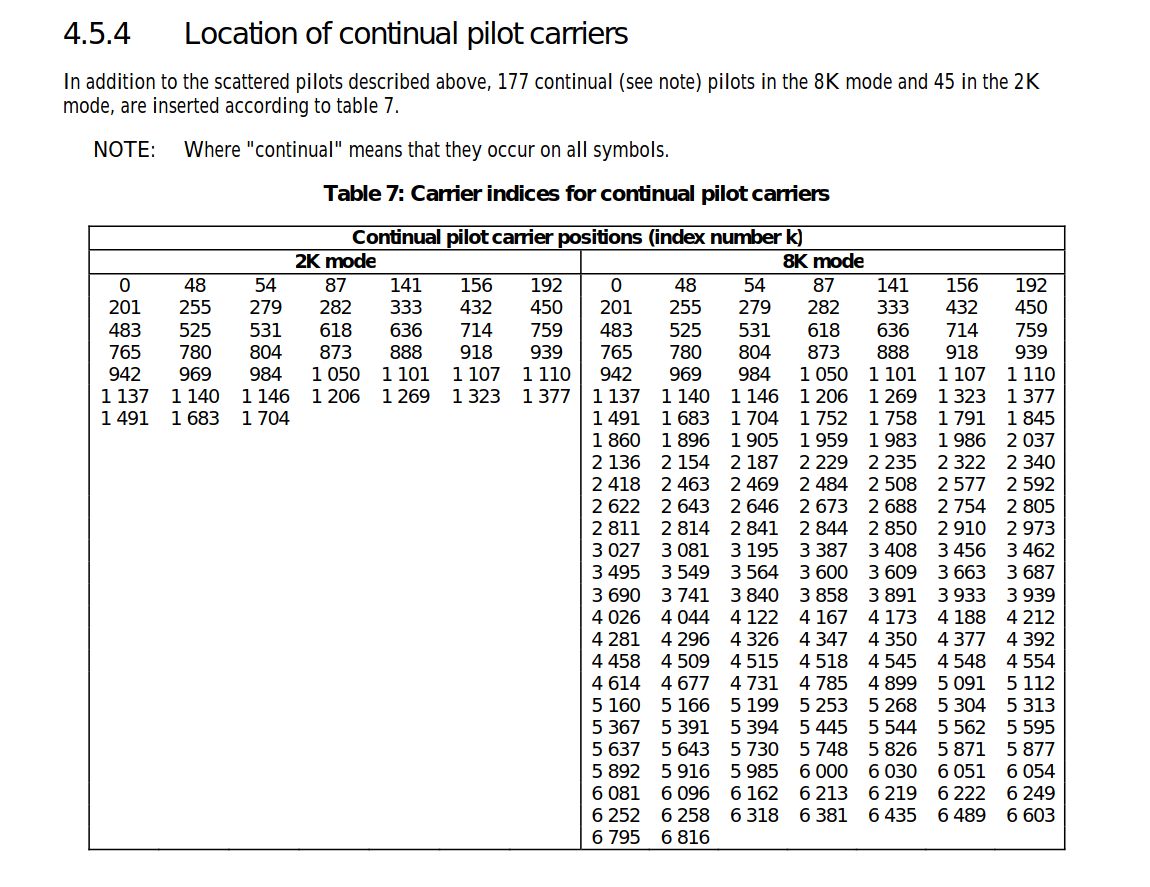
– continual pilot carriers;

– TPS carriers.

The modulation of all data cells is normalized so that E[c × c∗]= 1.

All cells which are continual or scattered pilots are transmitted at “boosted power level” so that for these E[c ×c∗] = 16/9.

The pilots can be used for frame synchronization, frequency synchronization, time synchronization, channel estimation, transmission mode identification and can also be used to follow the phase noise.

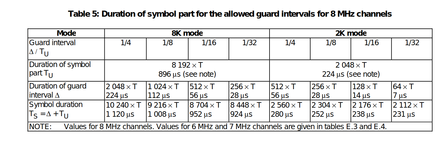
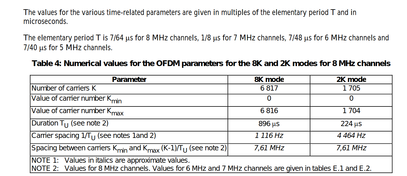
The carriers are determined by Kmin = 0 and Kmax = 1 704 in2K mode and 6 816 in 8K mode respectively. The spacing between adjacent carriers is 1/TU while the spacing between carriers Kmin and Kmax are determined by (K-1)/TU.

The numerical values for the OFDM parameters for the 8K and2K modes are given in tables for 8 MHz channels, for 6 MHz and 7 MHz channels.

We would collect some continual pilots and average them to get an overall current frequency. We would create an array of all the indexes of the continual pilot and use it.

Then we would subtract them with the known frequency of DVB-T. Hence, we would have the PPM shift. So that’s much of what we are doing for our tool.

It’s more interesting to work on once done with the boring Research work.

Anonymous Developer

Links –

Link to working repository is – https://github.com/AerospaceResearch/CalibrateSDR/tree/dvbt

I am attaching a test file too for a better understanding of this tool. Test file

Some more paper –

https://ca.rstenpresser.de/~cpresser/tmp/dvbt_7_paper.pdf

https://www.ese.wustl.edu/~nehorai/paper/Radar_Harms.pdf

http://ntur.lib.ntu.edu.tw/bitstream/246246/200704191002918/1/01258670.pdf

More Chat on-

https://www.linkedin.com/in/ayush-singh-101/

https://aerospaceresearch.zulipchat.com/#narrow/stream/281823-CalibrateSDR/topic/Signal.3A.20DVB-T

[GSoC2021] CalibrateSDR GSM Support – first coding period

Introduction

CalibrateSDR developed by Andreas Hornig is working perfectly with signals DAB+. We can use the python program to calibrate SDR devices. As part of the Google Summer of Code, I have been working around GSM Signal Standard to make CalibrateSDR compatible with it.

Before moving on, please read the initial blog on using CalibrateSDR, written by our mentor. The primary focus of this project is to extend the applicability towards more signal standards, so as to make it helpful for the SDR community. As DAB+ is mainly used in Europe, Signal standards like GSM, LTE, NOAA-Weather Satellites (use their sync pulses within the data) can be used.

Currently, it uses the pyrtlsdr package, which makes it work with RTL-SDR. Piping the API to work with other SDRs will also make the project have a wide range of applications in the SDR Community.

My first weeks of coding relied generally on implementing GSM signals. Working with the GSM frequency correction channel to calculate the offset is my primary task.

Proposed final working of CalibrateSDR

Working of GSM to calibrate the SDRs

GSM uses time division to share a frequency channel among users. Each frequency is divided into blocks of time that are known as time-slots. There are 8 time-slots that are numbers TS0 – TS7. Each time slot lasts about 576.9  μs. The bit rate is 270.833 kb/s, a total of 156.25 bits can be transmitted in each slot.

Each slot allocates 8.25 of its „bits time“ as guard-time, split between the beginning and the end of each time slot. Data transmitted within each time slot is called a burst. There are several types of bursts.

„Frequency correction“ burst, which is a burst of a pure frequency tone at 1/4th the bitrate of GSM or (1625000 / 6) / 4 = 67708.3 Hz. By searching a channel for this pure tone, we can determine its clock offset by determining how far away from 67708.3Hz the received frequency is.

How is it working?

A more robust way is to implement a hybrid of the FFT and filter methods. We could use the adaptive filter as described in the paper: G. Narendra Varma, Usha Sahu, G. Prabhu Charan, Robust Frequency Burst Detection Algorithm for GSM/GPRS (https://ieeexplore.ieee.org/document/1404796)

After finding the position of FCCH bursts that we receive in SDRs, it will be easy to calculate the offset. We measure it by how much shifted is the FCCH burst, than what we expect, that is at 67708.3 Hz from the frequency centre. Simply, if no offset is there, we could see these tone bursts at 67708.3 Hz offset with respect to the centre frequency of the channel.

I have completed the program to output the channel frequencies from the given ARFCN numbers of GSM. Check the code for the same here.

Detect and visualize the FCCH bursts!


Currently, the program has been tested only with IQ Wav file recordings. Even though the code has been designed to work with RTLSDR sticks, it is not tested yet with a live connection. Find the link to test files here.

After cloning the repo locally, run the setup to install the requirements using the command: python setup.py install

To test with GSM files, run:

python cali.py -m gsm -f <location of wav file> -rs <sampling rate> -fc <frequency center>

First, we will get the plot of the average power spectrum plot. Play with the code to increase the N value, and you can see the sharpness of the line.

The figure above shows the TDMA frames generated by the GSM Signal.

To determine the FCCH bursts from the signal, plot the spectrogram, using the function present in gsm.py. The spectrogram_plot function will do the fft and outputs the figure.

The generated FCCH bursts detection can be visualized as shown below:

We can see the pure tone FCCH bursts are occurring at specific intervals and can be visualized as small blue dots at a range of 0.25 from the centre.

Thus implementation of a filter bank and calculating the positions of these FCCH bursts will give us the offset frequency since we know these FCCH bursts occur at a distance of 67708.3 Hz from the frequency centre.

Will update the code after testing with gsm channels, and the function to calculate the final frequency offset will be committed to the repo.

The workarounds for the second coding period are implementation of LTE and NWS as well as the bridging of a more generalised SDR API, SoapySDR API, which has Python bindings to use as well.

Find out the project updates in my branch here: https://github.com/aerospaceresearch/CalibrateSDR/tree/jyrj_dev

References:

[GSoC2021: findsatbyrf] Summary of the first 5 weeks

By Binh-Minh Tran-Huu on 2021-07-15

  1. Introduction

Because of the recent sharp growth of the satellite industry, it is necessary to have free, accessible, open-source software to analyze satellite signals and track them. To achieve that, as one of the most essential steps, those applications must calculate the exact centers of the input satellite signals in the frequency domain. My project is initiated to accommodate this requirement. It aims to provide a program that can reliably detect satellite signals and find their exact frequency centers with high precision, thus providing important signal analysis and satellite tracking statistics.

  1. Overview

The project aims to locate the exact centers of given satellite signals with the desired accuracy of 1kHz, based on several different methods of finding the center. At first, the center-of-mass approach will be used to determine the rough location of the center. More algorithms will be applied from that location depending on the type of the signal to find the signal center with higher accuracy. 

Currently, for many NOAA signals, with the center-of-mass and “signal peak finding” approach (that will be shown below), we can get results with standard errors less than 1 kHz. For example, with the following signal, the standard error is 0.00378 kHz.

  1. Theoretical basis

The overall flowchart

  1. Fast-Fourier Transform (FFT)

Fourier Transform is a well-known algorithm to transform a signal from the time domain into the frequency domain. It extracts all the frequencies and their contributions to the total actual signal. More information could be found at Discrete Fourier transform

Fast-Fourier Transform is Fourier Transform but uses intelligent ways to reduce the time complexity, thus reducing the time it takes to transform the signal.

  1. Noise reduction and background signal reset

There is always noise in actual signals, but generally, noise has two important characteristics: normally distributed and its amplitude does not change much by frequency. You can see the signal noise in the following figure:

If we can divide the signal in the frequency domain into many parts such that we are sure that at least one of them contains only noise, we can use that part to determine the strength of the noise.

For example, consider only this signal segment:

By taking its average, we can find where the noise is located relative to the amplitude 0. By subtracting the whole signal to this average, we can ensure the noise all lies around the zero amplitude.

Next, we want to reduce all the noise to zero. To do that, we consider the distribution of noise, which is a normal distribution.

Photo from Characteristics of a Normal Distribution.

From this distribution, we are sure that 99.9% of noise has an amplitude less than three times the noise standard deviation. If we shift the whole signal down by 3 times this standard deviation, 99.9% of the noise will have amplitude less than 0.

From there, we can just remove every part of the signal with an amplitude less than zero. Then we will be able to get a signal without noise with the background having been reset to 0. 

You can clearly see the effect of this algorithm by looking at the signal of PIXL1 satellite above, where all the noise has been shifted to below 0.

  1. Center-of-mass centering

This algorithm is simple, the centroid position is calculated as (sum of (amplitude x position)) / (sum of amplitude), similar to how we calculate the center of mass in physics. The result of this algorithm is called the spectral centroid, more information could be found at Spectral centroid.

  1. Peak finding.

For signals with clear peaks such as APT(NOAA), finding the exact central peak points of the signal would give us good results. From the rough location of the center by the Center-of-mass method, we can scan for its neighbor to find the maximum peak. This peak will be the center of the signal that we want to find. 

For APT signals, this peak is very narrow, therefore this method is able to give us very high precision.

  1. Predicted signal centers from TLE

TLE (Two-line element set) information of a satellite can be used to determine the position and velocity of that satellite in the orbit. By using this data of position and velocity, we can calculate the relativistic Doppler effect caused by the location and movement of the satellite to calculate the signal frequency that we expect to receive on the ground.

  1. Error calculation.

Assume TLE gives us the correct result of signal center, we can calculate the standard error of the result by calculating the standard deviation:

Where n is the number of samples, x_i is the difference between our calculated center frequency from .wav and the frequency we get from TLE.

  1. Implementation in code:

https://github.com/aerospaceresearch/findsatbyrf/tree/bm_dev

  • main.py is where initial parameters are stored. The program is executed when this file is run.
  • tracker.py stores the Signal object, which is the python object that stores every information about a signal and the functions to find its center.
  • tools.py contains the functions necessary for our calculation and the TLE object used for center prediction.
  • signal_io.py stores functions and objects related to the input and output of our signal.
  1. Current results: For APT(NOAA):

Standard error = 0.00378 kHz

  1. Usage instruction:
    1. Create a folder with the name of your choice in the ‘findsat’ folder, for example, ‘data’.
    2. Put the .wav file of your signal in this folder with any name. 
    3. Put a satellite.tle file in the folder containing the TLE of your satellite.
    4. Put a station.txt file in the folder containing the name and location of the ground station where you recorded the signal separated by a “=”, for example (The numbers should be in degrees and meters):
    5. Change the content of main.py as instructed in the code, then run main.py. The result will be put in your ‘data’ folder.

name = Stuttgart

long = 9.2356

lat = 48.777

alt = 200.0

Example of station.txt

Future improvements

  • Enable running the program directly from the command line instead of opening a python file before running.
  • Add more methods to find the signal centers for other signal types.

Demonstration of the code. This type of video consumes too much memory therefore it is not used anymore, but this function could be reintroduced in the future.

Code demonstration