[GSoC’18|VisMa|Shantanu] Week #06-07: Finding the Unknown

This is GSoC’18 log#03. Here I will cover on what I have done in week#06-07. Link to the previous log.

Done so far…

I have implemented a simple solver which is capable of solving a given variable in terms of other variables and numbers. Below is a simple example of how the solver works.

„[GSoC’18|VisMa|Shantanu] Week #06-07: Finding the Unknown“ weiterlesen

[GSoC2018|OrbitDeterminator|Jorge] Week #5-6 – Implementation of Gauss method for Earth satellites and NEAs

Angles-only orbit determination: implementation of Gauss method

During these weeks, I worked towards implementing Gauss method for preliminary orbit determination using only angle measurements of a celestial body, either for Sun-centered (heliocentric, e.g., asteroids, comets, planets) or Earth-centered (geocentric, e.g. artificial satellites, space debris) orbits. Gauss method is able to take, for a given celestial object, only three pairs of right-ascension and declination observations, as seen from the surface of Earth, and compute an orbit from only those three observations.

In order to implement Gauss method, I followed closely the text from Howard D. Curtis, „Orbital Mechanics for Engineering Students“, specially section 5.10. For more details about the math behind the method, the reader is referred to this book.

The core idea and implementation

Gauss method may be summarized as follows: if we know the geodetic latitude phi_deg, the altitude above the reference ellipsoid altitude_km, the flattening of the Earth f; and if we have a list of three right ascensions ra_hrs and three declinations dec_deg associated to an observed celestial object, as well as the local sidereal time associated to those three observations lst_deg, and the time elapsed between them t_sec, then we are able to compute the cartesian state of the celestial body, referred either to the Sun or to the Earth, depending on the nature of its orbit. Here, we note that each one of ra_hrs, dec_deg, lst_deg and t_sec are lists with exactly three elements. Also, we note that the right-ascension and the declination determine the line-of-sight (LOS) of the celestial object with respect to the observer. Thus, we are able to write a function like this:

def gauss_method(phi_deg, altitude_km, f, ra_hrs, dec_deg, lst_deg, t_sec)
and the output of this function is the cartesian position r2 = [x,y,z] and the cartesian velocity v2 = [u,v,w] of the object, at exactly the time of the second observation.

A crucial detail

The output of Gauss method depends crucially on finding the real, positive roots of an 8-th order univariate polynomial, which is solved by means of Newton’s method in the book; we tested this using scipy.optimize.newton, but we actually obtained better numerical stability using numpy.roots, which allows to obtain the roots of an univariate polynomial of arbitrary finite order. One drawback of this method is that, in case of obtaining more than one real, positive roots to the polynomial, then one has to choose manually the root which corresponds to the physical motion of the object. But once the adequate root has been chosen, then the Gauss method gives a very good first estimate of the orbit.

Iterative refinement of Gauss method

Also, the output from the Gauss method may be refined; this involves computing iteratively better and better estimates of the Lagrange functions associated to the cartesian states at the first and third observations, in terms of the cartesian state at the second observation. Again, following the text from the book, we were able to implement the iterative refinement procedure for Gauss method.

Results

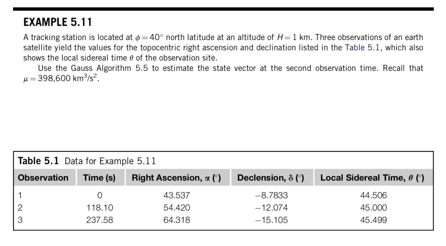
In order to test our code, we followed step-by-step the Examples 5.11 and 5.12 from the „Orbital Mechanics…“ book by H.D. Curtis.
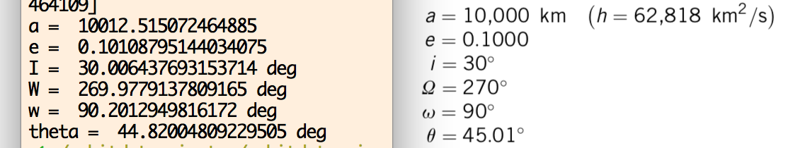
Our results closely follow the numbers cited by the author, although with some small differences, which we attribute to roundoff errors:
Regarding the refinement procedure (Algorithm 5.6), our results show convergence to practically the same values as the ones cited in the book:
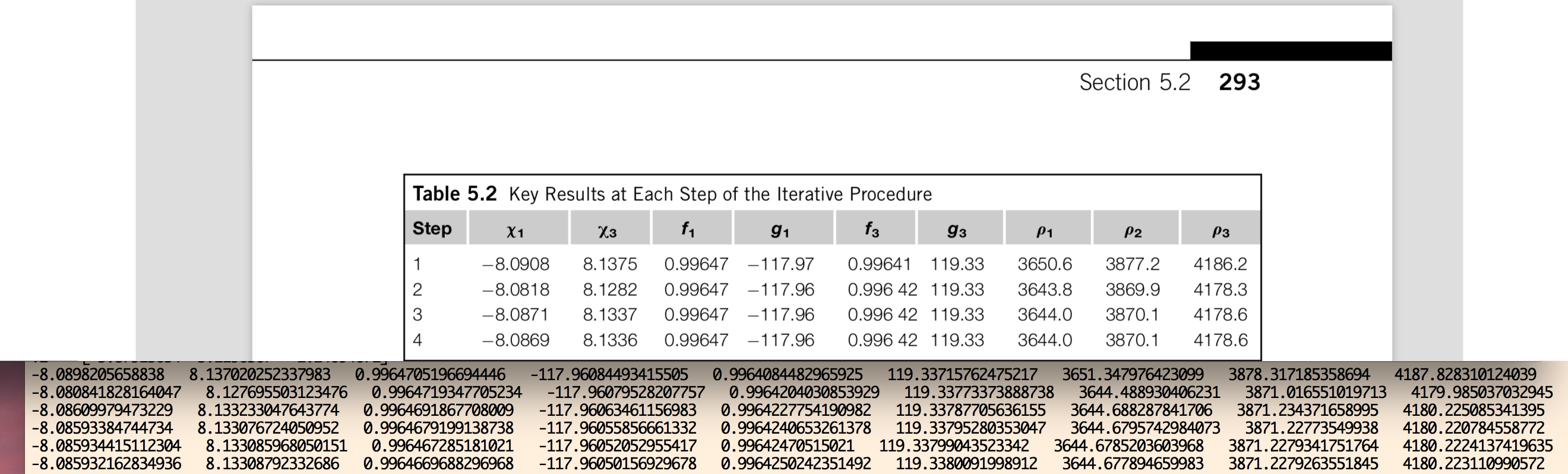
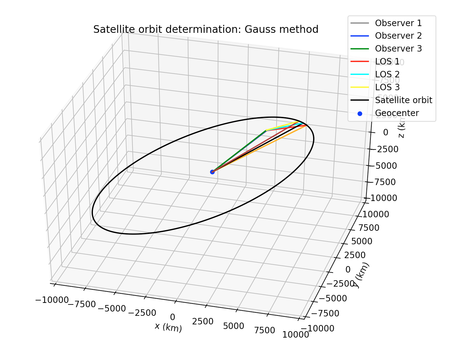
In the figure above, we show a comparison of the numbers we get for each of the quoted variables in the book, for each stage of the refinement iterative procedure for Gauss method. Although some small differences appear, eventually after about 15 to 20 iterations, our code shows convergence up to the precision of 64-bit floating point arithmetic. In the figure below, we show (black) the elliptic orbit corresponding to the output of Gauss method, for the observational data given in Example 5.11 from the book. The „Observer 1“, etc., lines correspond to the geocentric position of the observer on the surface of the Earth; „LOS 1“, etc., correspond to the line-of-sight vectors from the observer to the satellite defined by the RA-dec observations. The orange, black and brown lines correspond to the geocentric cartesian states of the satellite at the time of each observation, computed by means of the Gauss method.
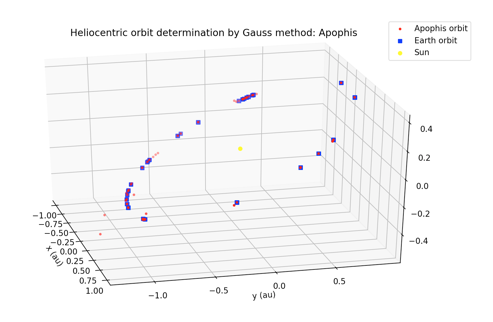
As a second test for our implementation of Gauss method, we took the observational data from the Minor Planet Center (MPC) for asteroid 99942 Apophis, which is a Near-Earth asteroid (NEA). Some differences with respect to Earth-centered orbits are: instead of km for length units and seconds for time units, it is better to use au (astronomical units) and SI days as length and time units, respectively. Besides, instead of the mass parameter μ=G*m for the Earth, we must use the Sun’s mass parameter (in au³ day¯² units). But one of the main differences of Sun-centered orbits with respect to the Earth-centered orbits, is that in order to compute the position of an observer on the surface of the Earth with respect to the center of the Sun, we must know in advance the position of the center of the Earth with respecto the center of the Sun. In order to achieve this, the Python package jplephem  was used, which allow us to retrieve the cartesian state of the center of the Earth wrt to the center of the Sun using the NASA-JPL DE430 planetary and ephemerides.
In the figure below, we show a processing of around 1,000 observations of Apophis, from various observatories from around the world, and using our implementation, we were able to reconstruct the orbit of the asteroid around the Sun:
Since the orbit of this asteroid suffers perturbations from the planets, as well as non-gravitational perturbations (e.g., Yarkovsky effect), then a direct application of Gauss method gives only a preliminary estimation of its orbit. In order to compute a more accurate orbit, this method has to be combined with other orbit determination methods (e.g., least-squares, etc.).

[GSoC2018|OrbitDeterminator|Arya] Week #5-6 – Making a DGSN simulator

This week I worked on propagating the satellite state. The NORAD TLEs are supposed to be used with the SGP4 propagator. It takes care of major perturbations like the oblateness of the Earth and atmospheric drag. Right now, Aakash is working on making one for our organization. But until then, I decided to work with the SGP4 module by Brandon Rhodes.

Working with SGP4

To make the code, I thought in reverse. We wanted to propagate a state vector from one time to another. So our function should look like this:

def propagate_state(r,v,t1,t2)

I checked and saw that the module only accepts TLEs as input. So we have to convert r,v to keplerian elements. Then artificially generate a TLE and input it to the module. The Celestrak website specifically asks us not to do this. But when data is not available, one must make approximations. I followed this approach and made the function successfully. However, I wasn’t satisfied. Artificially generating TLEs (which are strings) is computationally expensive. I wanted a direct way to feed the input. So I studied the source code and made another function that does the job without resorting to strings.

To propagate the state, we need to set the following parameters:

whichconst, afspc_mode,
inclo, nodeo, ecco, argpo, mo, no,
satnum, ndot, nddot, bstar,
epochyr, epochdays, jdsatepoch, epoch

The first line has constants which have default values. whichconst is the gravity model which is wgs72 by default. And afspc_mode is False unless you are dealing with old TLEs.

The second line has paramters that can be set directly from keplerian elements. The elements in order are inclination, longitude of ascending node, eccentricity, argument of periapsis, mean anomaly and number of orbits in a day.

The third line has parameters which are available in TLEs but they are not available to us. I set satnum, ndot and nddot to 0. satnum is irrelevant for the calculation. And ndot and nddot are normally very close to 0. For the bstar term, I couldn’t set it to zero because that would disable drag simulation. So I went through the b* terms of many satellites and got an average value of b* = 0.21109x10⁻⁴. Unless a b* term is supplied, this is used for the simulation.

The last line has parameters related to the epoch. These paramters in order are epoch year, day of year, julian date of epoch, and a Python datetime object of the epoch. These can be set by converting the epoch into a datetime object and manipulating it.

After putting together all this, you get the propagator:

The propagator in action.

The DGSN Simulator

Until the real DGSN comes online, we must work with a simulator. A live simulator will also allow us to make live predictions of the satellite. I thought that just running the propagator in an infinite loop will do the job. But it turned out to be more difficult. In a real time infinite loop, I can’t pause to take input. So I can’t control it while it’s running (like stopping or resuming it). Therefore I resorted to multi-threading. The main thread is used for controlling the program and calculations are done on another thread.

First, I made a basic simulator. It just prints the current location of any satellite, given it’s state at some previous time. There is a speed setting for development purposes too. The demo below is printing the position of the ISS every second in cartesian coordinates.

Next step was to add noise and gaps. Gaps are periods when no signal is available from the satellite. Adding noise was very easy. A random value between -15 and 15 kms is added to every component of the position vector. To add randomness in time, the time period between each observation is randomly decided. Implementing gaps was tougher.

I thought about it and deduced that gaps will be caused when the antenna can’t see the satellite. This will be caused by the rotation of the Earth and the revolution of the satellite. So the gaps will be periodic with time. To implement this, I wrote the following algorithm:

omega = <frequency>

p = abs(sin(omega * t))
if (p >= <threshold>):
    # process the output
    # as if the satellite is
    # within range
else:
    # continue as if the satellite
    # is out of range

The figure below shows the working of this algorithm:

By changing omega, one can control the frequency of the gaps. By changing threshold, one can control the duration of the gaps. A lower threshold means smaller gaps and vice-versa.

Putting it all together, I ran the simulator for 2 full orbits and plotted the results on the webapp I made last week. The results look pretty satisfying. 🙂

Next Steps

In the next couple of weeks, I will be tackling one of the hardest things in my proposal – the Kalman Filter. The Kalman Filter will take predictions from SGP4 and observations from real life/DGSN simulator and combine them to give more precise outputs. To do this first we have to synchronize the two streams of data (model and observations). Then we have to make the actual filter and pass the inputs through it. After that, we have to update the state in such a way that the filter can be used again. That’s a lot of work, so I am looking forward to a very exciting week ahead! 🙂

[GSoC2018|DirectDemod|Vinay] Week #5-6: NOAA-APT image extraction & AFSK1200 signal decoding

In my last blog we were at a point where we were able to detect the sync locations in NOAA signal. In this blog, we will look at  how the image is extracted and corrected. We will also have a brief look over the AFSK1200 decoder implemented by Andreas Hornig.

„[GSoC2018|DirectDemod|Vinay] Week #5-6: NOAA-APT image extraction & AFSK1200 signal decoding“ weiterlesen

[GSoC2018|VisMa|Shantanu] Week #03-05: Integrating the Integrator

This is GSoC log#02 (view log#01 here). Here I will cover on what I have done in week #03-05 and a gist of what has been accomplished in Phase I coding period.

Done so far …
  • Created parser.py which handles conversion of tokens to LaTeX or strings and vice-versa.
  • Some simplification issues were fixed
  • Integrated the differentiation.py and integration.py to the project along with the step-by-step explanation.
  • Support for partial differentiation and „partial integration“ was added.
  • The code was again refactored to decrease complexity and remove unused modules.
  • Added factorize.py module. Can currently factorize polynomials.

„[GSoC2018|VisMa|Shantanu] Week #03-05: Integrating the Integrator“ weiterlesen

[GSoC2018|DirectDemod|Vinay] Week #3-4 : NOAA-APT signal decoding

In my last blog  the process of accurately extracting sync locations within the NOAA APT signal was explored. In this blog, I would like to extend the comparison of the two methods that were implemented. Then look at how the process is influenced by presence of noise, sample drops and doppler effect.

„[GSoC2018|DirectDemod|Vinay] Week #3-4 : NOAA-APT signal decoding“ weiterlesen

[GSoC2018|OrbitDeterminator|Arya] Week #3-4 – Ground Track and WebApp for OrbitDeterminator

We got important stuff done in weeks 3 and 4. Everybody knows that visuals and graphics are very important for presentation purposes. The most popular library for plotting is matplotlib. It can generate excellent plots but in the end, they are static images. Instead of static images it’s better if some interactive content is presented. So we decided to make a webapp for OrbitDeterminator. A webapp makes it easier for the end-user to run the program. It can also be hosted on a publicly-accessible server, which means that anyone can use it without going through the pain of downloading and installing the program. For making the webapp, my mentor Alexandros suggested the excellent Dash library by Plotly.

Dash by Plotly

Dash is a Python library that can be used to make web applications. The library is built to be hosted on a server and be used by multiple people at once. It is powered by Plotly which produces beautiful, interactive plots in the browser itself. Programming in Dash is simple. First, you have to define the layout of the app in the form of a list of html components. You can style them as you like or add additional parameters. After this, you have to define callback functions. These functions will be triggered whenever the user interacts with the UI (like pressing a button, or typing some text). These functions can be used to change the elements displayed on the app. This makes the app interactive.

Designing the app

For now, OrbitDeterminator’s primary function is to find a good set of orbital elements that match a noisy set of observations. The webapp will be a graphical way to do this. Observations are stored in CSV files in the following format:

# Comments
# here.
#
# t x y z
<time_1> <x_1> <y_1> <z_1>
<time_2> <x_2> <y_2> <z_2>
...
<time_n> <x_n> <y_n> <z_n>

So the webapp must have a place to upload csv files. We also want to show the name of the file and the file contents in case the user has uploaded the wrong file. And of course, we have to show the results and plots of the results. After discussing with Alexandros, I settled on this layout:

  • File upload box
  • File name and contents
  • Keplerian elements
  • Spatial plots
  • Ground track
  • Coordinate vs time plot
  • Residuals plot

But the user might not require all this information at once. So all the components must be collapsible, to hide them from view if not required. Making the webapp required lots of googling but was relatively easy. The end result is this:

OrbitDeterminator Webapp

All the plots are interactive. You can zoom, pan, and rotate them. You can also save any plot you want as a png file. Most of the plots were straightforward. The most difficult plot was the ground track, whose algorithm I will discuss below.

Plotting the ground track of a satelllite

To plot the ground track, we have to know the position of the satellite with respect to the Earth’s surface. First, I thought that just converting the coordinates into polar form and plotting φ vs θ would do the job. But I forgot that the satellite coordinates were measured with respect to an inertial (fixed) reference frame, whereas the Earth’s surface is rotating. So the actual coordinates will be different. I went through two articles on CelesTrak and Astronomy StackExchange to come up with the algorithm.

NORAD uses True Equator Mean Equinox (TEME) reference frame for its TLEs. In this frame, the origin is at the Earth’s centre. The z-axis points toward the North Pole. The x-axis points to the vernal equinox. And the y-axis completes the right-handed coordinate system.

TEME Coordinate System

We need to convert coordinates in TEME to an Earth-Centered-Eath-Fixed (ECEF) reference frame. In such a frame, the origin is at the Earth’s centre and the the coordinate axes are fixed to the Earth’s surface (which means that they rotate along with the Earth). Many such frames exist but the standard one is the International Terrestrial Reference Frame (ITRF). In this frame, the z-axis points toward the North Pole, the x-axis points toward 0°E 0°N. And the y-axis completes the coordinate system. Since both TEME and ITRF share a common z-axis, the latitude will not be affected. Only the longitude will be shifted by a certain amount. This amount, known as the Earth Rotation Angle, is the angle between TEME’s x-axis and ITRF’s x-axis. Now I will write down the pseudocode I used to determine this angle.

Let t be the time at which we want to find the Earth’s rotation. Let t_mid be midnight on the same day, so that t - t_mid is the UTC time during the day. Let J2000 be the time Jan 1 2000 12:00 pm UTC(this is the J200 epoch). Then the pseudocode is:

days_since_J2000 = t_mid - J2000
# multiply the above by an appropriate 
# constant to convert the units into days

# centuries since J2000
Tu = days_since_J2000/36525

# effects of precession of the Earth's axis
tg0h = 24110.54841         +
     8640184.812866 * Tu   +
           0.093104 * Tu^2 -
           6.200e-6 * Tu^3

# Greenwich Mean Siderial Time in seconds
tgt = tg0h + 1.00273790935 * (t-t_mid)

# rotation angle in degrees
rotation_angle = (tgt%86400)*360/86400

After getting the rotation angle, we can subtract it from θ to get the actual longitude.

Putting everything together , we get this plot of the ISS for 21st May 2018 18:27:54 UTC. I used this NASA website to generate the NASA ISS plot.

Ground Track of the ISS on 21st May 2018 from 18:27:54 for 2 orbits.
Ground Track of the ISS as generated by OrbitDeterminator
Ground Track of the ISS as generated by NASA.

As you can see, the results line up pretty well. Note that this is a simplified model and is not super-accurate, but it gives roughly the same results.

Future Work

  • Integrating the SGP4 model into OrbitDeterminator.
  • Making a DGSN simulator (this will be used until the real DGSN starts working).
  • Making a Kalman filter to combine the two sources of data.

[GSoC2018|USOC GUI|Pedro] Weeks 3-4 – Handling Protocol Data

This is my second post since the start of GSoC18. I would recommend you check my first post for a bit of context before reading this.

Current state of the project

I spent the past two weeks designing a new Window for assigning variables defined in a protocol file anytime during runtime of the application. This feature is one of the main goals/tasks of my project during these 3 months as a GSoC student, so I don’t want to rush a definitive solution.

For a little insight, a protocol file is a XML file that tells the Ground Station how incoming data should be handled. It contains multiple sensors, each one with different variables and datatypes. Before, the selected protocol was hardcoded which means that the user would have to compile and re-run the application for the changes to take effect. This was fixed in my first implementation of the Layout Creator Window in the first two weeks. Now, there’s the need of assigning data from the protocol to the created charts and states. My first solution for this problem was an ‚Assign Data‘ Button inside each chart/state in the LayoutCreator window.

Assign Data Button
Assigning Data to a Chart

After some time, i figured this would not be the optimal solution for many reasons:

  • The user may not want to assign variable information to UI components right away.
  • If there is a big number of charts and states, assigning variables to each one becomes time-expensive and tedious.
  • There’s no way of knowing which variables and sensors are assigned to each chart. The user would have to open each component’s window and check.
  • No support for dragging and dropping variables (another project requirement)

All of these above go against what was proposed right at the beginning: a quick and simple implementation of a ground station that lets the user focus on what’s important, rather than the User Interface.

So, I came across another design and solution for this. Instead of assigning variables to a chart/state one at a time, all desired charts and segments are shown inside a TreeView.

Assigning Data to Charts/States

By selecting a variable from the left TreeView (source) and a state/chart from the right TreeView(destination), the user can easily assign data to UI components. For now, a button click is needed to shift variables from one tree to another, but I plan on implementing a drag-and-drop‘ feature in the future.

Protocol data persistence

Last dev blog I talked about how GUI preferences are being stored in a JSON file. To avoid having to handle protocol data each time the user loads an existing configuration file, I had to store some more information in the JSON file (protocol name, variables and sensors). For now, only the corresponding names are stored.

What’s next

There are still some bugs with the new iteration of the AssignDataWindow. It seems simple shifting variables from one tree to another, but since each item is treated as a String, there’s quite a lot of logic behind it to make sure the right components and variables are being correctly assigned. Besides, I still haven’t started working on actually assigning protocol data to charts and states (i need to make the layout creation process as solid as possible before that).

First month and evaluations

After 4 weeks of work, I finish my first coding period. I believe I achieved what I planned in my proposal for this time. I’ve been having a great time at this organization and I believe every other student feels the same. Our mentors are great and really want us to succeed more than anything. See you in two weeks!


– Pedro Portela

Four weeks at GSoC

About the Author: Hello guys, I am Aakash Deep. I am a B.Tech. student from Indraprastha Institute of Information Technology, Delhi (IIIT-D) in Computer Science and Engineering (CSE). I am a speed-cuber and obviously, my hobby is solving Rubik's Cube.

This post is in the continuation of my last post, as the last post contains the information about the first two weeks as being a GSoC student and the work done in that time frame. Those who missed it can access that post here.

Week 3 and 4

As the database was created earlier and now it is updating every day as the new TLEs are getting store into it. Now, the work left is implementing propagation model.

For the propagation algorithm, the SGP4 algorithm is used. The algorithm takes the TLE as input and computes position and velocity vectors. Now, we will come to the workflow of the code,  that how the code is behaving. A sample test file is added to my github (can be found here). The file contains the multiple TLEs of a single satellite which is taken from the database. The code takes this as input and passes it to the propagation model. Then propagation model computes the position and velocity vectors of each TLE. After that, the averaging occurs and in the end, we get a single position and velocity vector. These vectors are then used to find the orbital elements of the satellite.

Evaluation 1

Phase 1 evaluation of the GSoC is nearby. The dates of the deadline are from June 11 to June 15. Following checkpoints are met before the deadline:

  • Creating database
    Creating the database and a table for mapping satellite’s name to its corresponding md5 hexadecimal hash and initializing tables in the database for each satellite.
  • Scraping data from web
    Scrape data from the celestrak site and populated it into the database into their respective tables.
  • Maintaining database
    Updating database whenever new TLE comes on the website.
  • Implement Propagation Model
    Converting TLE into position and velocity vector and then computing orbital elements. Now, there can be two ways to do it.  We have a file containing multiple TLE of the same satellite at different time points.
    The first way is, feeding this file as input. Compute position and velocity vector of every TLE and average these vectors to get a single vector. Use this averaged vector to calculate orbital elements.
    The second way is, feeding the file as input. Compute position and velocity vector of each TLE and from these TLE calculate position and velocity vector for each pair of vector and then average the orbital elements. After this, we will get the averaged orbital elements.
    Right now, I don’t know which way is better but we as a team trying to figure it out.
  • Compute orbital elements
    Calculates orbital elements from the given pair of position and velocity vector.

Work on Progress

  • Documentation
  • Testing

[GSoC2018|OrbitDeterminator|Jorge] Week #3-4 – Least squares fit to cartesian positions as a function of time

Introduction

An orbital fit by least-squares is a technique for computing the set of six Keplerian elements which best describe an orbit with respect to a *whole* set of observations.
As the set of Keplerian elements we choose semimajor axis a, eccentricity e, time of perigee passage τ (i.e., how much time has elapsed since the last perigee), as well as the standard Euler angles which describe the orientation of the orbital plane with respecto to the inertial frame: argument of pericenter ω, inclination I and longitude of ascending node Ω. We denote by X the set of these six Keplerian elements; that is, X = (a, e, τ, ω, I, Ω).
A least-squares fit is simply to look the minimum of a scalar (i.e., real-valued) „cost“ function Q(X). The Q function is simply a measure of how well our theoretical predictions, for a given set X of orbital elements, depart from observations. In an ideal world, we could find a set of orbital elements such that it perfectly matched the observations and thus Q(X)=0. Nevertheless, real-world measures carry uncertainties, and we can only hope to find orbital elements X which make Q attain its minimum possible value with respect to all the observations we have made.
The values of the cost function Q(X) for a least-squared problem are constructed the following way: take *all* the values you observed (call them v_i), and substract from each of those the values you were expecting to measure for a given set of orbital elements X (say, V_i(X) ). Call each of these differences the residuals, xi_i(X) = v_i-V_i(X) . Then, square the residuals, and sum all the squared residuals. The value you obtain following this recipe, is the value of Q(X).
In practice, the least-squares method finds a local minimum of the cost function by performing an iterative procedure, which needs a good initial „guess“ solution X0; otherwise the procedure may converge to non-feasible results. Hence, it is necessary that the „good“ initial guess be provided by a preliminary orbit determination method.

„[GSoC2018|OrbitDeterminator|Jorge] Week #3-4 – Least squares fit to cartesian positions as a function of time“ weiterlesen