About the author: Hello everyone, I am Aakash Deep, I am a 4th year undergraduate student pursuing my degree in Bachelor's of Technology (B.Tech) in Computer Science and Engineering (CSE) from Indraprastha Institure of Information Technology, Delhi (IIIT-D) in India. I am a space enthusiast and I like travelling. My major hobby is speed-cubing.
About the organization
The organization for which I am working is AerospaceResearch.net. It has many interesting projects not only for the under-graduate beginners but for the masters‘ degree students too. We are a small group of enthusiasts who love to solve problems related to space. The benefit of being a part of a small group is that you get to know each other in a very short duration of time. We have regular meetings with our project mentors. The best part is that we can contact our mentors anytime. My mentor is Nilesh Chaturvedi who has guided me throughout the project and is still doing so. Alexandros Kazantzidis is also one of the mentors in the organization who cleared my doubts while building the propagation model.
Link to the organization repo.
Project
The title of the project is Implementing Two-Line Element (TLE) Input / Output and using it for evaluation.
What is TLE?
Two-Line Element (TLE) is a data format or a way of encoding various parameters of an object orbiting Earth at any particular time point, an epoch. TLEs can describe the trajectories only of Earth-orbiting objects. It is widely used as an input for projecting the future orbital tracks of space objects. A TLE set may include a title line preceding the element data, so each listing may take up three lines in the file. The title is not required, as each data line includes a unique object identifier code. The two lines contain a lot of information about the object and have a length of 69 characters each.
About Module
The scripts that were added to the module are database initialization, scraper, parser, Gibb’s method, and propagation model. More details about each element are as follows:
Database
Database contributes a major role in testing and generating the result of a module. In the beginning, we did not have TLE data. So, we decided that we will store TLEs from the celestrak website in the database. Now, it is time to choose which database we are going to use: SQL or NoSQL? Both the databases have their own advantages and disadvantages. After taking care of the needs and the data which we are going to store, we chose SQL based data. The reason behind this choice is that the input is well defined and structured. We only want to store 2 strings (that is, line 1 and line 2 of the TLE) at a particular time epoch. MySQL is used to store the data. The format of the data stored in the database is – timestamp, line 1 of TLE, line 2 of TLE.
For database creation, initialization, and maintenance two python scripts were written:
- initDatabase.py
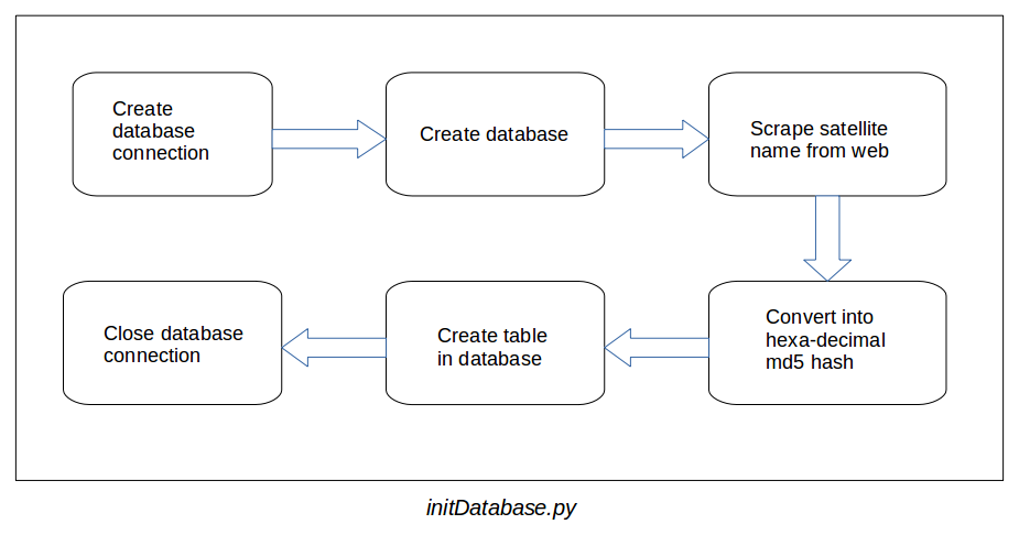
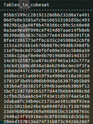
The script first creates a database in MySQL so that we can create tables to store the TLEs of the satellites. After that, it crawls the celestrak website and extracts the satellite names only, so that we can create tables in our database. But there was a problem in the creation of tables as the satellite names contain special characters (like dashes, spaces and parenthesis) and giving a special character into a MySQL command produced an error. To solve this problem, satellite names were converted into their respective hexadecimal md5 hash value which was an alphanumeric value and hence the problem was solved. So, the names of the tables are now satellite’s md5 hash value. The format of the tables inside the database is,+-----------+---------------+---------------+ | timestamp | line_1_of_tle | line_2_of_tle | +-----------+---------------+---------------+ | t1 | line1 | line2 | | t2 | line1 | line2 | | .. | ... | ... | | .. | ... | ... | | tn | line1 | line2 | +-----------+---------------+---------------+
The flowchart of the script is as follows,

Following is the image of the database containing the tables,

- scraper.py
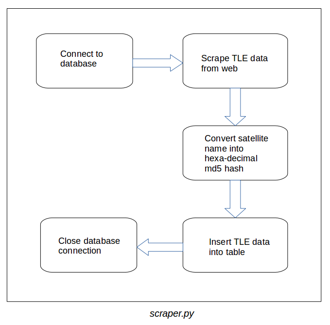
This script is responsible for updating/adding a new TLE data into the database. The script first creates a connection with the database and then crawls the celestrak website to extract TLE data for every satellite present there. After the data is extracted, it converts the name of the satellite to its md5 hash and adds the TLE data into the respective table through a MySQL query.
The flowchart of the script is as follows,

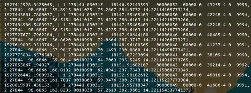
The table containing TLE data,

* Format of the table is given above
Currently, the database module is shifted from the organization repository to my own repository (which contains all the codes created during the GSoC) on github as it is producing a build error during the build process. In this build process (which was running on github), the script is creating a connection with the locally stored MySQL database which is then creating an error in it. The database module will be added later using some online database.
The database module can be found here.
Gibb’s Implementation
See the source code here.
Gibb’s method is based on the fact that two body orbits lie in a plane. It takes three position vectors as its input arguments and generates a pair of position vector and velocity vector, together known as the state vector. The Gibbs method is implemented using the OOP concepts and hence it supports the data abstraction and encapsulation. The method includes a lot of mathematical computation.
The input to the script is in the following format,
timestamp, x-coordinate, y-coordinate, z-coordinate
t1, x1, y1, z1
t2, x2, y2, z2
t3, x3, y3, z3
..
..
tn, xn, yn, zn
A pseudo-code and a brief explanation of the script is as follows,
Pseudo-code:

Note: Vector is in bold and magnitude is in normal format.
      e.g - 'a' represents vector and 'a' represents it's magnitude.

Input:
r1 - first position vector
r2 - second position vector
r3 - third position vector

1. Take r1, r2 and r3.
2. Calculate C12 = r1 x r2, C23 = r2 x r3 and
   C31 = r3 x r1.
3. Verify that û.Â23 = 0 (û is u cap or unit vector u)
4. Calculate N, D and S from below equations,
   N = r1(r2 x r3) + r2(r3 x r1) + r3(r1 x r2)
   D = r1 x r2 + r2 x r3 + r3 x r1
   S = r1(r2 - r3) + r2(r3 - r1) + r3(r1 - r2)
5. Calculate v2 from below,
   v = √(µ/ND) . ((D x r)/r + S)

Now, take r2 as position vector, v2 as velocity vector and both will together form state vector.
A brief explanation of the script
A file containing position vectors at various time epoch is passed into the script. The script reads the file and takes a set of three consecutive position vectors in order to apply the Gibbs method on it. The format of the file is – timestamp, x coordinate, y coordinate, z coordinate. After taking the set, the script passes the data into gibbs() function (pseudo code of Gibb’s Method is mentioned above). Then the function computes the result and returns the state vector. Next time the loop iterates, the first position vector gets removed from the set and the next position vector from the file gets added as the third position vector and it is then again passed into the function. As the file contains a lot of position vectors and for a set of 3 consecutive vectors, the script is generating a state vector. It is evident that the output generated will be two less than the total number of position vectors in the input file. After taking this point into consideration, a vector is created which stores every state vector into it and returns it as result.
Calculating orbital/keplerian elements
The script contains a function which converts the state vectors into Orbital or Keplerian elements namely semi-major axis, inclination, right ascension of the ascending node, eccentricity, argument of perigee, and mean anomaly which can thus help further in tracking and plotting satellite’s orbit and in a lot of other computation.
Pseudo code for converting state vector into orbital elements is as follows:
Pseudo Code:

Note: Vector is in bold and magnitude is in normal format.
      e.g - 'a' represents vector and 'a' represents it's magnitude.

Input:
r - position vector
v - velocity vector

1. Calculate the distance,
   r = √r.r
2. Calculate the speed,
   v = √v.v
3. Calculate the radial velocity,
   vr = r.v/r
4. Calculate the angular momentum and it's magnitude,
   h = r x v
   h = √h.h
5. Caculate inclination,
   i = cos–¹(hz/h)       | hz : z-axis in h
6. Calculate node line and it's magnitude,
   Ê = [0, 0, 1]
   N = Ê x h
   N =√N.N
7. Caculate right ascension of the ascending node,
         _
        |  cos–¹(Nx/N)          if (Ny ≥ 0)
   Ω = /
       \
        |_ 360° - cos–¹(Nx/N)   if (Ny < 0)
   where,
   Nx : x-axis in N
   Ny : y-axis in N
8. Calculate eccentricity vector,
   e = (1/µ)[(v² - µ/r)r - r.vr.v]
9. Calculate eccentricity,
   e =√e.e
10. Calculate argument of perigee,
         _
        | cos–¹(N.e/N.e)          if (ez ≥ 0)
   ω = /
       \
        |_ 360° - cos–¹(N.e/N.e)  if (ez < 0)
   where,
   ez : z-axis in e
11. Calculate true anomaly,
         _
        | cos–¹(e.r/e.r)          if (vr ≥ 0)
   θ = /
       \
        |_ 360° - cos–¹(e.r/e.r)  if (vr < 0)
12. Calculate semi-major axis,
    rp = h²/(µ.(1+e))       | µ : 398600.4418 (constant)
    ra = h²/(µ.(1-e))
    a = (rp+ra)/2
Propagation Model
See the source code here.
Simplified perturbations models are a set of five mathematical models (SGP, SGP4, SDP4, SGP8 and SDP8) used to calculate orbital state vectors of satellites and space debris relative to the Earth-centered inertial coordinate system. This set of models is often referred to collectively as SGP4 due to the frequency of use of that model particularly with two-line element sets produced by NORAD and NASA.
The propagation model used for the project is SGP4. The model takes a TLE without title line as input arguments. The output generated by the propagation model is a state vector.
A brief explanation of the script
The code is taking TLE as input. Then it extracts the necessary elements in compute_necessary_tle() from the TLE which helps in the computation of the SGP4. The necessary information includes inclination, right ascension of the ascending node, eccentricity, argument of perigee, mean anomaly, mean motion, and bstar drag term. After that, the propagation model is exected which include a lot of heavy mathematical computation. After the computation gets over, the function return state vector as output.
Now to check whether the code is producing the results correctly, we need to convert the resulted state vector into TLE back. So, one more function is added which recovers the TLE back from state vectors. To validate the result, Spacetrack Report 3 is used which contains a sample TLE to find the state vector at a particular epoch. The propagation model is taking two input arguments t1 (start epoch time) and t2 (stop epoch time). The resulting state vector is computed in the given range [t1, t2] (including both the points). As there is a state vector at every epoch so an output vector is created which stores all the state vectors and returns it as a result.
Now, the problem is that the input is coming in the form of Keplerian elements and the function accepts a TLE. One way to resolve this is to recover the TLE back from the Keplerian elements and then pass TLE as an input and again extract the same information (in compute_necessary_tle() function) in order to propagate the model. But since this approach is costly, the other way to resolve the problem is to create another function which takes Keplerian elements as input parameters. As a result, there is no need to transform the same information again and again. This is the reason why compute_necessary_kep() was added. Now, the code is accepting the input in both ways: keplerian elements as well as TLE. In other words, execution of the code can either start from compute_necessary_tle() or compute_necessary_kep() depending on the input. After producing state vectors from t1 to t2, the script is storing it into an array and returns it as an output.
Follow below steps to run the script:

>>> obj = SGP4()
>>> obj.compute_necessary_kep(<input>)
    or
>>> obj.compute_necessary_tle(<input>)
>>> obj.propagate(t1, t2)
Calling compute_necessary_kep() or compute_necessary_tle() is necessary. As this function extracts the important information from the given input and initializes the class variables which are further used in the propagation model and without which the computation will not be possible. If compute_necessary_kep() or compute_necessary_tle() is not called then the interpreter will throw a custom exception, which says,
Error: Call compute_necessary_kep() or compute_necessary_tle() function
       of the class SGP4 before calling propagate().

Function Declaration:

    compute_necessary_kep(list, float)
    Parameter 1:List of keplerian elements (semi-major axis,
                inclination, ascension, eccentricity, perigee, anomaly)
    Parameter 2:bstar drag term
    Returns: NIL

    compute_necessary_tle(str, str)
    Parameter 1: First line of the TLE
    Parameter 2: Second line of the TLE
    Returns: NIL
So, just remember to call the functions in the correct sequence and you are good to go.
A test file for propagation model is also written which verifies the output of the two functions propagation_model() and recover_tle().
Credits for Propagation Model
- Spacetrack Report No. 3 (Models for Propagation of NORAD Element Sets)
- MATLAB File Exchange SGP4
Important Links
- Commits: https://github.com/aerospaceresearch/orbitdeterminator/commits?author=aakash525
- Database: https://github.com/aakash525/Orbital-Determinator/tree/master/code/database
- Gibbs Method: https://github.com/aerospaceresearch/orbitdeterminator/blob/master/orbitdeterminator/kep_determination/gibbsMethod.py
- Propagation Model: https://github.com/aerospaceresearch/orbitdeterminator/blob/master/orbitdeterminator/propagation/sgp4.py