Overview:
This program finds the center in the frequency domain of a signal by time.
This is the link to its Github repository. There, you can also see the markdown (.md) file that contains the same content as this blog.
Every major work on this repository is done by Binh-Minh Tran-Huu under instructions and monitor from mentor Andreas Hornig of Aerospaceresearch.net as a project participated in Google Summer of Code 2021.
Usage:
Step 1: Prepare your wave file (.wav/.dat) and a json file containing the information about your signal
Example of the json file:
{
    "signal": {
        "name": "NOAA-18",
        "type": "NOAA",
        "center_frequency": 137.5e6,
        "time_of_record": "2021-06-04T20:17:05.00Z"
    },
    "tle": {
        "line_1": "1 28654U 05018A   21156.90071532  .00000084  00000-0  69961-4 0  9998",
        "line_2": "2 28654  98.9942 221.7189 0013368 317.9158  42.0985 14.12611611826810"
    },
    "station": {
        "name": "Stuttgart",
        "longitude": 9.2356,
        "latitude": 48.777,
        "altitude": 200.0
    },
    "default_channel": [
        {
            "frequency": 137912968,
            "bandwidth": 60e3
        }
    ]
}
Where:
- „signal“ object contains information about the signal file, such as name, center frequency and time of record. For now, there is only „type“: „NOAA“ is supported, if the signal is not NOAA then you should put „type“: null or simply remove that key.
- „tle“ object contains the two lines of the „two-line element“ file of the satellite that the signal comes from.
- „station“ object contains the information of the station, such as name, longitude (degree), latitude (degree) and altitude (meter).
- „default_channel“ object contains a list of channels that will be analyzed in case there is no channel input from the command line. It could handle more than one channel, you can always add more channels into that list, for example:
"default_channel": [
        {
            "frequency": 400574.350e3,
            "bandwidth": 20e3
        },
        {
            "frequency": 400575.0e3,
            "bandwidth": 20e3
        }
    ]
NOTE: „tle“ and „station“ objects are only needed if you intend to use signal center frequency prediction based on TLE, „default_channel“ object is only needed if you want to not put channel information into the command line, otherwise you can remove them.
Step 2: Run the program from the Command-Line Interface (CLI)
Simply use Python to run the file main.py with the following arguments:
[-h]
-f wav/dat_file
-i json_file
[-o name_of_output_file]
[-ch1 frequency_in_Hz] [-bw1 frequency_in_Hz]
[-ch2 frequency_in_Hz] [-bw2 frequency_in_Hz]
[-bw3 frequency_in_Hz] [-ch3 frequency_in_Hz]
[-ch4 frequency_in_Hz] [-bw4 frequency_in_Hz]
[-step time_in_second]
[-sen frequency_in_Hz]
[-filter float]
[-tle]
[-begin time_in_second]
[-end time_in_second]
With:
- -h: to show help.
- -f (required): to input the directory of the wave file.
- -i (required): to input the json signal information file.
- -o: directory and name without extension of the wanted output file, defaults to „./output“.
- -ch0, -ch1, -ch2, -ch3: to input the frequencies (in Hz) of up to 4 channels to be analyzed. Will overwrite the „default_channel“ provided by the json file.
- -bw0, -bw1, -bw2, -bw3: to input the bandwidth (in Hz) of up to 4 channels to be analyzed. Will overwrite the „default_channel“ provided by the json file.
- -step: to input the length in time (in second) of each time interval, defaults to 1.
- -sen: to input the sensitivity, which is the width of each bin in the frequency kernel (in Hz) after FFT, defaults to 1.
- -filter: to input the strength of the noise filter as ratio to 1. For example, filter of 1.1 means the noise filter is 1.1 times as strong, or 10% stronger than the default filter, defaults to 1.
- -begin: to input the time of begin of the segment to be analyzed, defaults to 1.
- -end: to input the time of end of the segment to be analyzed, defaults to the end of the file.
- -tle: used to turn on prediction based on Two-line elements (TLE) file, otherwise this function is off.
EXAMPLES:\
python3 .\main.py -i .\MySignal.json -f .\MySatellite\MySignal.wav -ch0 400.575e6 -bw0 20e3 -o D:\\CubeSat -begin 10. -end 60. -tle

python3 ./main.py -i /home/MyUser/MySignal.json -f ./MySatellite/MySignal.wav -ch0 400.575e6 -bw0 20e3 -o ./CubeSat

python3 ./main.py -i /home/MyUser/MySignal.json -f ./MySatellite/MySignal.wav -filter 1.25
Output:
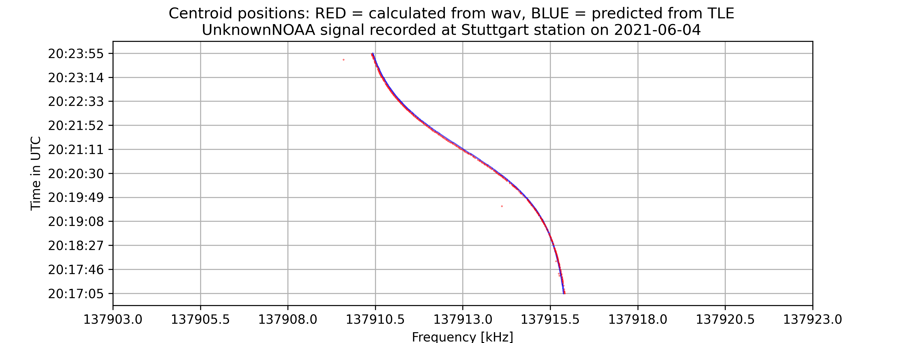
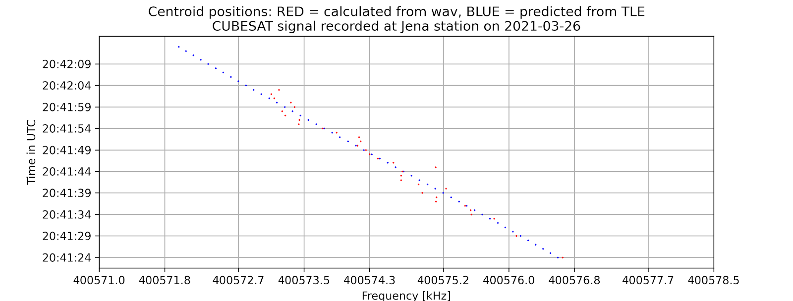
- A time vs. frequency graph, showing the center of the signal in the frequency domain by time, for example:
- A .csv file storing the center position in the frequency domain by time.
- A .json file with a „header“ object containing metadata of the signal and „signal_center“ object containing centers of the signal for each channel by time.
- On the command-line interface, if -tle is enabled, there will be information about the offset between the calculated frequencies from the wave file and from the tle file as well as the standard error of the signal compared to prediction.

All files are exported with name and directory as selected with the [-o] argument.
Test files:
You can use the files here to test the code.
Description:
1. Introduction:
Because of the recent sharp growth of the satellite industry, it is necessary to have free, accessible, open-source software to analyze satellite signals and track them. In order to achieve that, as one of the most essential steps, those applications must calculate the exact centers of the input satellite signals in the frequency domain. My project is initiated to accommodate this requirement. It aims to provide a program that can reliably detect satellite signals and find their exact frequency centers with high precision, thus providing important statistics for signal analyzing and satellite tracking.
2. Overview
The project aims to locate the exact centers of given satellite signals with the desired accuracy of 1kHz, based on several different methods of finding the center. At first, the center-of-mass approach will be used to determine the rough location of the center. From that location, more algorithms will be applied depending on the type of the signal to find the signal center with higher accuracy. Currently, for many APT/NOAA signals, with the center-of-mass and “signal peak finding” approach (that will be shown below), we can get results with standard errors less than 1 kHz. For example, with the example signal above, the standard error is 0.026 kHz.
3. Theoretical basis
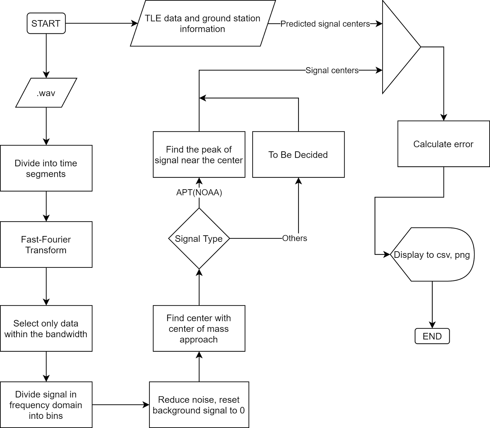
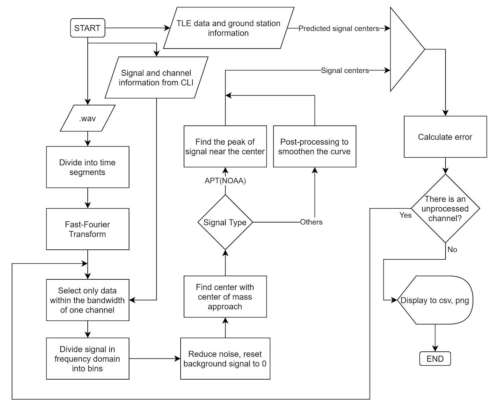
The overall flowchart:
- Fast-Fourier Transform (FFT)
Fourier Transform is a well-known algorithm to transform a signal from the time domain into the frequency domain. It extracts all the frequencies and their contributions to the total actual signal. More information could be found at Wikipedia: Discrete Fourier transform.
Fast-Fourier Transform is Fourier Transform but uses intelligent ways to reduce the time complexity, thus reducing the time it takes to transform the signal.
- Noise reduction and background signal reset:

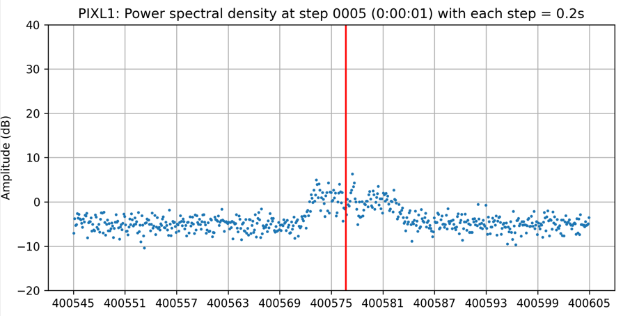
In actual signals, there is always noise, but generally noise has two important characteristics, which is normally distributed and its amplitude does not change much by frequency. You can see the signal noise in the following figure:
If we can divide the signal in the frequency domain into many parts such that we are sure that at least one of them contains only noise, we can use that part to determine the strength of noise.
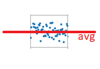
For example, consider only this signal segment:

By taking its average, we can find where the noise is located relative to the amplitude 0. By subtracting the whole signal to this average, we can ensure the noise all lies around the zero amplitude.
Next, we want to reduce all the noise to zero. To do that, we consider the distribution of noise, which is a normal distribution.
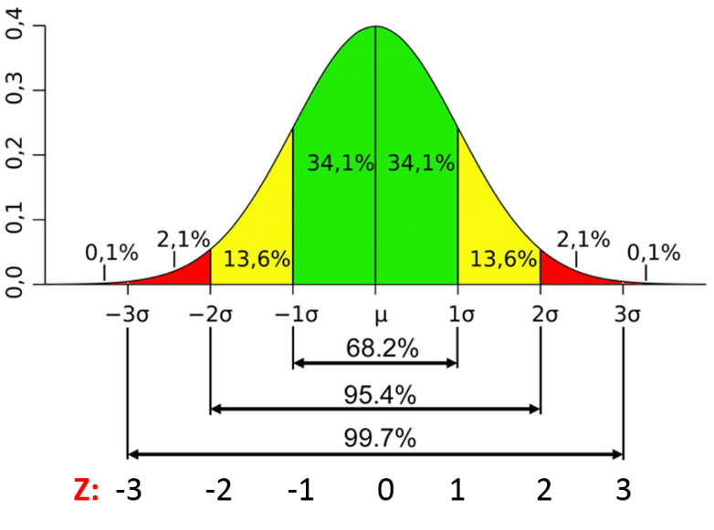
From this distribution, we are sure that 99.9% of noise has amplitude less than three times of the standard deviation of noise. If we shift the whole signal down by 3 times this standard deviation, 99.9% of the noise will have amplitude less than 0. From there, we can just remove every part of the signal with an amplitude less than zero. Then we will be able to get a signal without noise with the background having been reset to 0.
You can clearly see the effect of this algorithm by looking at the signal of PIXL1 satellite above, where all the noise has been shifted to below 0.
- Center-of-mass centering
This algorithm is simple, the centroid position is calculated as: (sum of (amplitude x position)) / (sum of amplitude), similar to how we calculate the center of mass in physics. The result of this algorithm is called the spectral centroid, more information could be found at Wikipedia: Spectral centroid.
- Peak finding.
For signals with clear peaks such as APT(NOAA), finding the exact central peak points of the signal would give us good results. From the rough location of the center by Center-of-mass method, we can scan for its neighbor to find the maximum peak. This peak will be the center of the signal that we want to find. For APT signals, this peak is very narrow, therefore this method is able to give us very high precision.
- Predicted signal centers from TLE
TLE (Two-line element set) information of a satellite can be used to determine the position and velocity of that satellite on the orbit. By using this data of position and velocity, we can calculate the relativistic Doppler effect caused by the location and movement of the satellite to calculate the signal frequency that we expect to receive on the ground. For more information, visit Wikipedia: Relativistic Doppler effect.
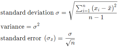
- Error calculation. Assume TLE gives us the correct result of signal center, we can calculate the standard error of the result by calculating the standard deviation:

Where n is the number of samples, x_i is the difference between our calculated center frequency from .wav and the frequency we get from TLE.
4. Implementation in actual code:
- main.py is where initial parameters are stored. The program is executed when this file is run.
- tracker.py stores the Signal object, which is the python object that stores every information about a signal and the functions to find its center.
- tools.py contains the functions necessary for our calculation, as well as the TLE object used for center prediction.
- signal_io.py stores functions and objects related to the input and output of our signals and instructions.
5. Current results:
- For APT(NOAA): Standard error = 0.004 kHz
- For PIXL1(CUBESAT): Standard error = 0.029 kHz

6. Potential further improvements:
- Expand the program to work better with more types of signals.
- Make video-output function works with reasonable computing resources.
Currently, with my private version of the code, I am able to make videos such as this one, but it took too much time and memory to actually make one, therefore I did not put it into the official code.