Introduction
An orbital fit by least-squares is a technique for computing the set of six Keplerian elements which best describe an orbit with respect to a *whole* set of observations.
As the set of Keplerian elements we choose semimajor axis a, eccentricity e, time of perigee passage τ (i.e., how much time has elapsed since the last perigee), as well as the standard Euler angles which describe the orientation of the orbital plane with respecto to the inertial frame: argument of pericenter ω, inclination I and longitude of ascending node Ω. We denote by X the set of these six Keplerian elements; that is, X = (a, e, τ, ω, I, Ω).
A least-squares fit is simply to look the minimum of a scalar (i.e., real-valued) „cost“ function Q(X). The Q function is simply a measure of how well our theoretical predictions, for a given set X of orbital elements, depart from observations. In an ideal world, we could find a set of orbital elements such that it perfectly matched the observations and thus Q(X)=0. Nevertheless, real-world measures carry uncertainties, and we can only hope to find orbital elements X which make Q attain its minimum possible value with respect to all the observations we have made.
The values of the cost function Q(X) for a least-squared problem are constructed the following way: take *all* the values you observed (call them
v_i), and substract from each of those the values you were expecting to measure for a given set of orbital elements X (say, V_i(X) ). Call each of these differences the residuals, xi_i(X) = v_i-V_i(X) . Then, square the residuals, and sum all the squared residuals. The value you obtain following this recipe, is the value of Q(X).In practice, the least-squares method finds a local minimum of the cost function by performing an iterative procedure, which needs a good initial „guess“ solution
X0; otherwise the procedure may converge to non-feasible results. Hence, it is necessary that the „good“ initial guess be provided by a preliminary orbit determination method.
Implementation
We consider the concrete case of having m observations of the cartesian coordinates of the position vector (x,y,z) referred to the center of attraction (the Earth for artificial satellites, or the Sun for asteroids, etc.) at a given time t. That is, for a time t1 we have (x1,y1,z1); for t2 we have (x2,y2,z2); etc.
For this particular case, we assumed the motion to be Keplerian and we wrote the function
orbel2xyz, which takes as arguments the time t, the mass parameter mu (mu =G × m) of the center of attraction, the semimajor axis a, the eccentricity e, the time of pericenter passage tau, the argument of pericenter omega, the inclination I and the longitude of ascending node Omega. The output of orbel2xyz is the expected value at time t of the cartesian positions x, y, z, for a given set of orbital elements. The cartesian position vector is returned as a 1-dim numpy.array of length 3. Is is constructed by first computing, from the time, the corresponding true anomaly by inverting the Kepler equation n(t-τ)=E-e · sin(E) using a modified version of Newton’s method, as described by Murray and Dermott in their book „Solar System Dynamics“; our implementation is focused on both accuracy and speed and is able to invert Kepler’s equation in 5 iterations to almost machine accuracy, even for high eccentricities (for details, see `time2truean` and related functions). Then, as a second step, we compute the position of the observed object in its orbital frame using standard formulae (this was done in function xyz_orbplane_). Finally, using the Euler angles omega , I and Omega, we rotate from the orbital frame to the inertial frame using the orbplane2frame_ function. This allows us to compute our predicted values for the observations, which were denoted by V_i(X) in the previous section.The next step is to retrieve the observed values
v_i from a data file. We do this using the numpy.loadtxt function.The vector of residuals
xi_i is computed via the res_vec function, which takes as input the set of orbital elements x as well as a 2-dim numpy.array called my_data , as well as the mass parameter of the Earth in appropriate units, my_mu_Earth . Note that if the lengths are, for example, in meters and the times in seconds, then the Earth’s mass parameter has to be given in meters³/seconds².Next, the cost function Q is automatically optimized using the
scipy.optimize.least_squares function, taking as input the res_vec function, an initial guess for the orbital elements x0 , the complementary arguments for the res_vec function which in this particular case are the input data data and the mass parameter of Earth mu_Earth . First I thought of using the scipy.optimize.minimize function; but SciPy’s least_squares function was chosen because of its access to the Levenberg-Marquardt algorithm, which is quite robust for this kind of problems. The method for nonlinear least squares fitting was the Levenberg-Marquardt algorithm. The output of the least_squares function is a data structure labeled as Q_ls, which among other things, provides the solution to the least-squares problem for the given observational data and associated parameters.Results
Some results are presented using the
determine_kep method from ellipse_fit . For the example file orbit.csv , we see an improvement of more than 25% with respect to the initial orbit. Even though the orbital elements are corrected by relatively small quantities, it is sufficient to get a 25% better solution for the orbital elements, in the sense that the cost function attains a lower value with respect to the initial set of elements.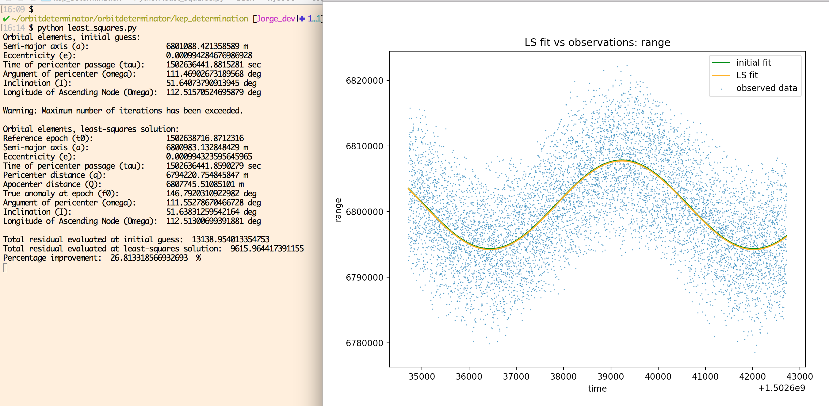
Discussion and future work
Using well established tools, an implementation of a least-squares orbital determinator for the case of t,x,y,z data was implemented. In preliminary tests, we see improvements of around 25% with respect to existing methods. Although execution times are around a couple of seconds, the obtained improvement helps increase the accuracy of the fitted orbital elements, which is essential to orbit propagation.
Furthermore, although the particular scenario of having observed values of t,x,y,z might not be of general use, the tools developed here will help attain least-squares orbit determinators for objects which are observed with optical instruments (telescopes) and range/range-rate radar astrometry. Indeed, using the code what has been done in this work, it will be feasible to construct an orbit fitter which will handle optical observations. To achieve this, the immediate solutions which must be provided to handle, for example, the optical observations case are the following:
- Conversion from topocentric right ascension/declination to geocentric equatorial celestial coordinates.
- Computation of atmospheric aberration to optical observations.
- Correction for light-time travel.
- Allow for non-homogeneous weighting of observations in least-squares (i.e., insert weights in residuals-computing function).
- A preliminary orbit determinator for optical observations which will seed the least-squares fitter (e.g., Gauss‘ method).