After the implementation of the Cowell propagator, it was time for the Kalman Filter. It is an algorithm that uses a series of measurements observed over time, containing statistical noise and other inaccuracies, and produces estimates of unknown variables that tend to be more accurate than those based on a single measurement alone. A Kalman Filter is the ideal filter for a linear process having Gaussian noise. Since our process is not linear, a modified version of the filter must be used. This is called the Extended Kalman Filter. It linearizes about the point in question and applies the regular Kalman Filter to it.
To apply the filter, the following things are required:
- A function f which outputs the next state, given the current state.
- The matrix F which is the jacobian of f .
- The matrix H which converts state into corresponding observations.
- A matrix Q denoting process noise. It consists of the inaccuracies in the model.
- A matrix R denoting measurement noise.
The variables involved during the calculations are:
- x – the state of the system
- z – the observations of the system
- P – covariance matrix of x. It denotes the inaccuracy in the estimate. As the filter runs, P is supposed to decrease.
- K – the Kalman gain. This matrix is between 0 and I and denotes how much the observations can be trusted vs how much the model can be trusted.
The filter consists of two major steps:
- Predict – in this step, we predict the next state (x) and covariance matrix (P) using our model.
- Update – in this step, we update our estimates of x and P using observations (z).
The equations of the filter are:
Predict:
Update:
The filter has to be initialized with a value of x and P. If the initial value of P is not known, it can be set to an arbitrary large value.
My implementation
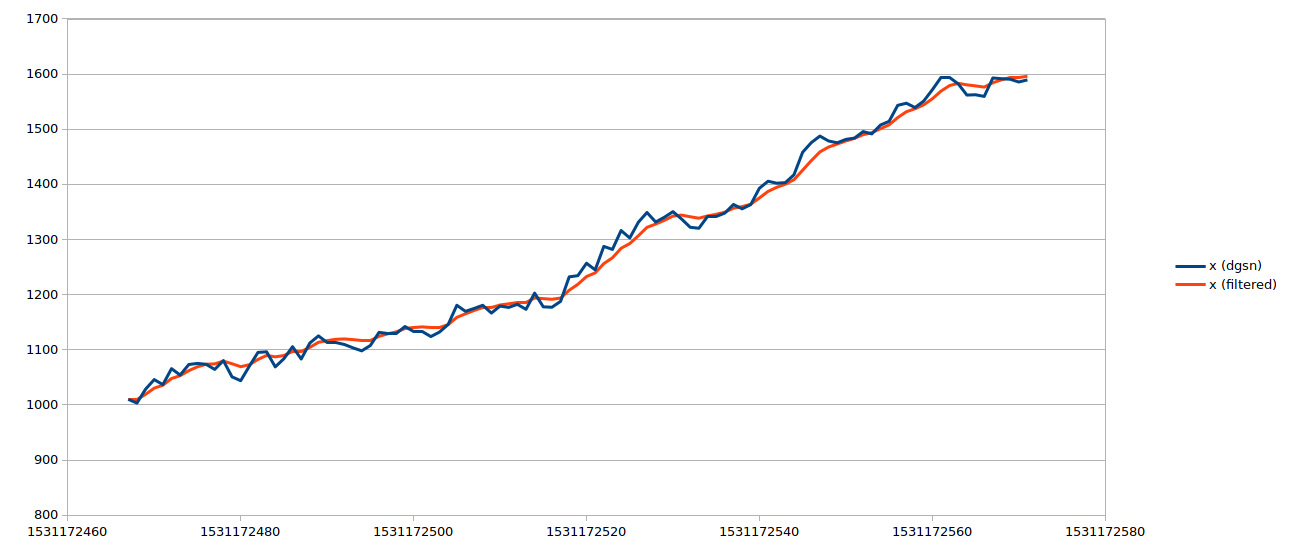
Currently there is a doubt about whether the DGSN will be able to supply complete velocity information at any time. Hence, I left out velocity from the computation and only focused on the position. Therefore x is the position vector. f in this case is rk4(_,t1,t2). To find F I numerically found out the Jacobian of f with a step size of 0.0005 km. I set Q and R as diagonal matrices with constant values of 10 km and 30 km respectively. Since we are directly getting the coordinates from DGSN, h is the identity function and H is the identity matrix H. I initialized P as a diagonal matrix with large values. Then I ran the filter and after it converged it started giving out smoother values.
Possible simplifications
I observed that for short intervals of time, F is approximately equal to the identity matrix. Since computing the Jacobian is expensive, we can set F equal to I for short periods. For long periods since observations are to be trusted more, we can set x to z directly. I also observed that P is approximately equal to a scalar times I. Making these simplifications will transform the matrix equations into scalar ones:
Predict:
Update:
If q and r are constants then we can further simplify the equations to find the final steady state Kalman Gain k and covariance p:
The simplified equations become:
Predict:
Update:
Possible improvements
Of course, the simplifications highlighted above are only possible because our covariance matrices are too simple. Some possible improvements are:
- Use time varying Q and R matrices. After a long interval of no measurements, the uncertainity in position is higher. So Q should be larger, and vice-versa.
- Try to include velocity into the state. Right now, we are not sure whether the DGSN can measure all the 3 components of velocity at an instant, but we know that it will be able to measure one component using Doppler shift. Thus we can try to incorporate it into the filter using a time-varying R matrix.
References
- https://vtechworks.lib.vt.edu/bitstream/handle/10919/49102/Keil_EM_T_2014.pdf
- https://en.wikipedia.org/wiki/Extended_Kalman_filter
- https://en.wikipedia.org/wiki/Kalman_Filter