Autor: Arya Das

Introduction

OrbitDeterminator is part of the bigger DGSN project by AerospaceResearch.Net. The Distributed Ground Station Network will be a network of thousands of ground stations across the globe. Together, these ground stations will track satellites cheaper and faster than conventional tracking stations. It will also get ordinary citizens involved in real space missions, so it is a win-win for everybody.

The purpose of OrbitDeterminator is to process the data coming from the DGSN and estimate the orbit of the satellite. It should also be able to predict the satellite’s location at any future time. This is the approximate workflow of the project:

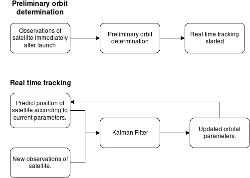
(Note that the project is still under development so this workflow might change in future.)

My mentor was Alexandros Kazantzidis. He alongwith Nilesh Chaturvedi had worked on the preliminary orbit determination part last year. However the results could be improved. So I worked a little on that, but my main contribution was on real time tracking. As a side project I made a web application for one of the modules. I also cleaned the repo by adding a gitignore file and removing all temporary and IDE files.

Technical Details

The project is hosted on GitHub and made entirely in Python. It includes a requirements.txt and setup.py file. So it can be installed easily using pip. The project directory structure is quite simple and intuitive:

├── docs
└── orbitdeterminator
    ├── example_data
    ├── filters
    ├── kep_determination
    ├── propagation
    ├── test_deploy
    ├── tests
    └── util

Observation data is stored in the form of csv files in the following format:

# the data consists of 4 columns separated by spaces:
#
# time, x-coordinate, y-coordinate, z-coordinate
#
# for example:

1526927274 -5234.47464 4126.08971 -1266.52201
1526927284 -5272.8012 4094.65453 -1208.06841

Time is stored in unix timestamp format. Unit of distance (unless otherwise specified) is a kilometer. Keplerian orbital elements are stored in the form of a 1×6 numpy array:

kep[0] = semi-major axis
kep[1] = eccentricity
kep[2] = inclination
kep[3] = argument of perigee
kep[4] = right ascension of ascending node
kep[5] = true anomaly

Similarly, state vectors are stored in the form of a 1×6 numpy array:

s = [rx,ry,rz,vx,vy,vz]

This should be enough to get one started. For more help you can check the documentation.

Preliminary Orbit Determination (blog post)

Last year two methods of filtering were developed – the Savitzky-Golay filter and the Triple Moving Average filter. Two methods of orbit determination were also developed – the Lambert’s method and an interpolation method. However, they were not giving good results for certain kinds of data.

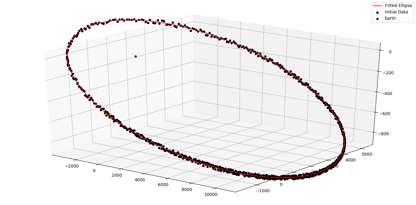
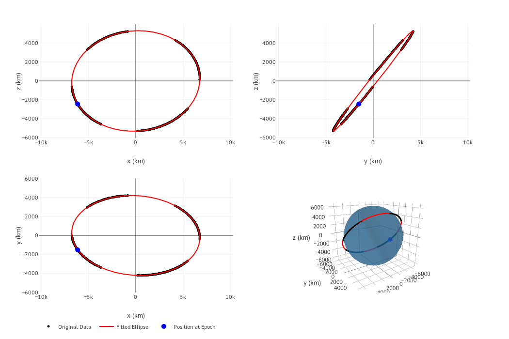
I made a new algorithm that fits an ellipse to the data, similar to fitting a line to a set of points. It gave better results than the previous algorithms so we decided to continue with it.

Propagation (blog post)

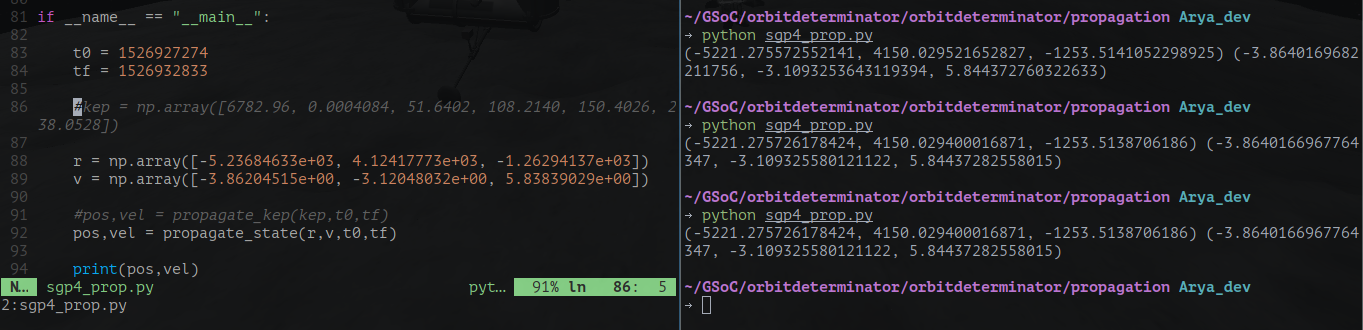
The real time tracking consists of two parts – propagation of state vector and the Kalman filter. For propagation we decided to use the SGP4 algorithm. It did the propagation excellently but was not stable with the Kalman filter. So I made a simple propagator. It uses numerical integration and takes into account atmospheric drag and the oblateness of the Earth. After making it I spent a lot of time testing it. The only major problem was that the time period did not match with the real time period. A simple fix for this was to manually fiddle with the semi-major axis of the satellite until it gives the correct time period. I tried a lot to fix this problem, but could not do so. Anyway, since it was working well with the Kalman filter, we decided to continue.

DGSN Simulator (blog post)

Since enough ground stations do not exist yet, we need some sort of artificial data to test the Kalman filter with. So I proposed to make a DGSN simulator module. The basic idea was that it will give the location of the satellite periodically with some noise. In the end the simulator had the following features:

• Noise in spatial coordinates
• Non-uniform interval between observations
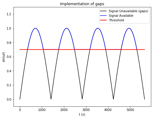
• Gaps in observations (to simulate the satellite being out of range)
• Simulation speed control

The simulator in action. It is printing the coordinates every second.

Plotting the data produced by the simulator.

Kalman Filter (blog post)

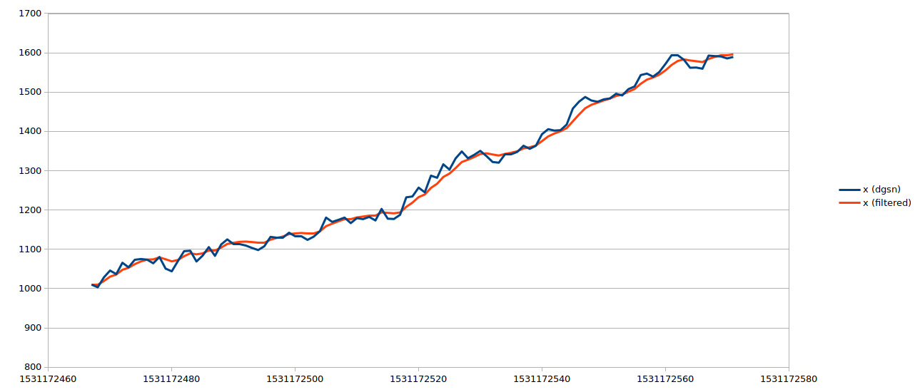
After all this the Kalman filter was left. This was quite straight-forward. I directly implemented the equations on Wikipedia and it worked quite well. However if a time varying covariance matrix is used, it will give better results.

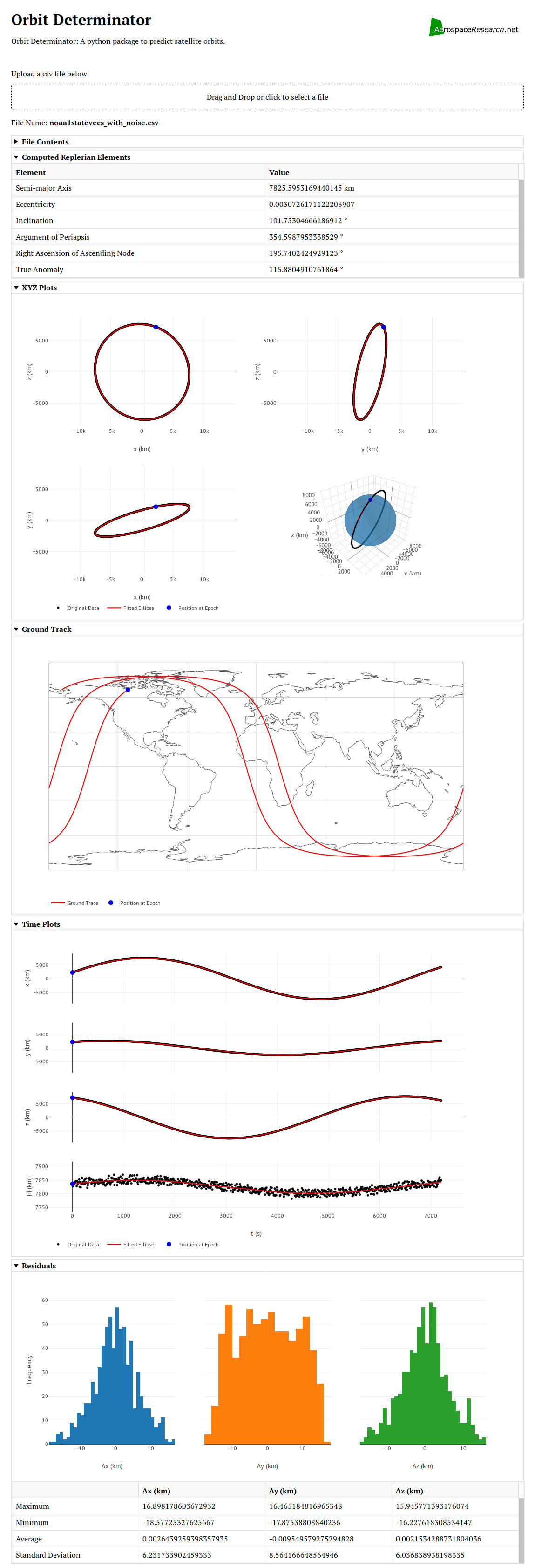
Web Application (blog post)

As a side project I made a web application for the ellipse fit algorithm. We created a new repository for this because it is not a necessary component of orbitdeterminator. It is made using the Dash library. Upload a csv file, it will process and give the orbital elements alongwith beautiful graphs.

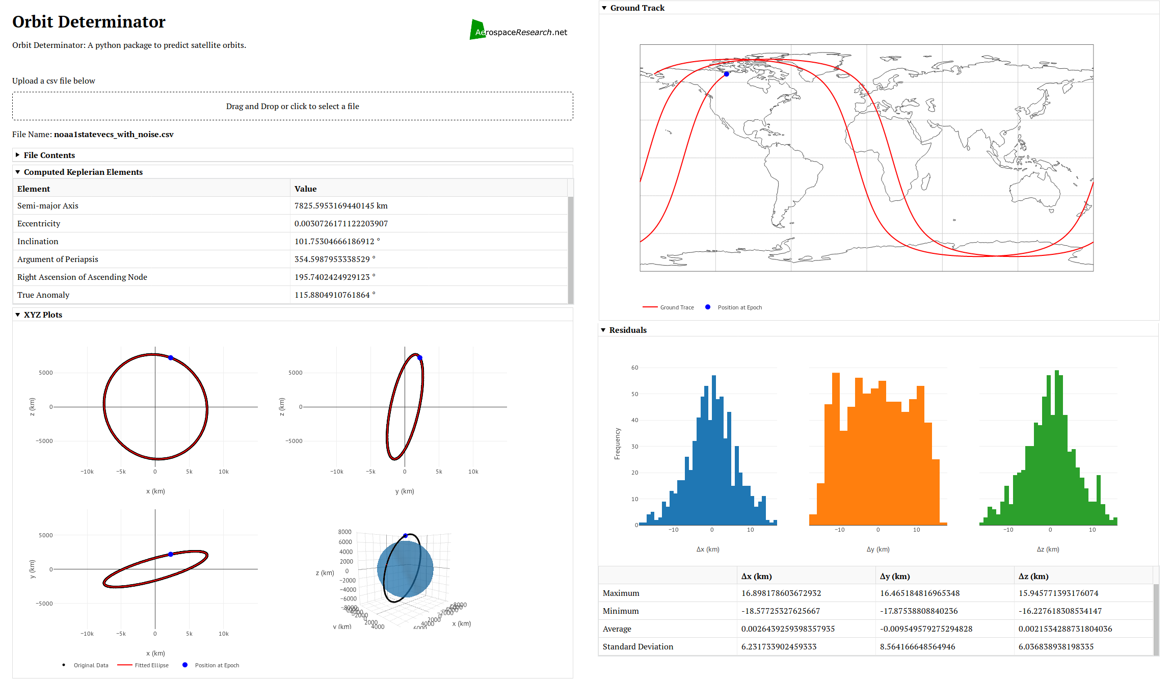
The web application

List of scripts I created

• kep_determination/ellipse_fit.py
• propagation/cowell.py
• propagation/simulator.py
• propagation/dgsn_simulator.py
• propagation/kalman_filter.py
• propagation/sgp4_prop.py
• propagation/sgp4_prop_string.py
• tests/test_ellipse_fit.py
• util/anom_conv.py
• util/new_tle_kep_state.py
• util/teme_to_ecef.py
• orbitdeterminator-webapp/app.py

Future Work

• Integrating Aakash’s SGP4 module with the Kalman filter.
• Fixing the time period problem in the numerical propagator.
• Testing the system with real observations.
• Improving the Kalman filter.
• Deploying the web application on a public server.

Useful Links

• Source code
• Documentation
• My commits
• My blog posts
• Distributed Ground Station Network
• AerospaceResearch.Net

After the implementation of the Cowell propagator, it was time for the Kalman Filter. It is an algorithm that uses a series of measurements observed over time, containing statistical noise and other inaccuracies, and produces estimates of unknown variables that tend to be more accurate than those based on a single measurement alone. A Kalman Filter is the ideal filter for a linear process having Gaussian noise. Since our process is not linear, a modified version of the filter must be used. This is called the Extended Kalman Filter. It linearizes about the point in question and applies the regular Kalman Filter to it.

To apply the filter, the following things are required:

• A function f which outputs the next state, given the current state.
• The matrix F which is the jacobian of f .
• The matrix H which converts state into corresponding observations.
• A matrix Q denoting process noise. It consists of the inaccuracies in the model.
• A matrix R denoting measurement noise.

The variables involved during the calculations are:

• x – the state of the system
• z – the observations of the system
• P – covariance matrix of x. It denotes the inaccuracy in the estimate. As the filter runs, P is supposed to decrease.
• K – the Kalman gain. This matrix is between 0 and I and denotes how much the observations can be trusted vs how much the model can be trusted.

The filter consists of two major steps:

• Predict – in this step, we predict the next state (x) and covariance matrix (P) using our model.
• Update – in this step, we update our estimates of x and P using observations (z).

„[GSoC2018|Orbitdeterminator|Arya] Week #8-9: Implementing Kalman Filter“ weiterlesen

Last time when we tried to use the SGP4 propagator in our Kalman Filter, we ran into problems. This was because you can’t stop the algorithm at a certain stage and continue from there. Suppose you want to propagate from to , you can directly propagate from to but you can’t propagate it from to to . So I set out to make our own propagator taking into account two major perturbations – oblateness of Earth and atmospheric drag. Instead of making an analytical propagator like SGP4, I went with a numerical one because that can be stopped and started at any point. So the first challenge was making a numerical integrator.

Numerical Integration

Numerical integration are used to integrate a differential equation from one point to another point. I studied and tested various integrators and finally settled on Runge-Kutta 4th order integrator (RK4).

Advantages of RK4:

• Good accuracy for small to medium step sizes
• Low computation cost
• Easy to implement

Let the initial value problem be and .

Choose a step size and define

for  where,

Note that these equations work equally well whether y is a scalar or a vector. In our case, the differential equation is . It is not in a form suitable to be used directly in RK4. To use it in RK4 we have to vectorize the equation. First, let’s define the state of the system as . Let . Then,

This form can be directly used in the RK4 integrator.

„[GSoC2018|OrbitDeterminator|Arya] Week #7-8: Implementing Cowell propagator“ weiterlesen

This week I worked on propagating the satellite state. The NORAD TLEs are supposed to be used with the SGP4 propagator. It takes care of major perturbations like the oblateness of the Earth and atmospheric drag. Right now, Aakash is working on making one for our organization. But until then, I decided to work with the SGP4 module by Brandon Rhodes.

Working with SGP4

To make the code, I thought in reverse. We wanted to propagate a state vector from one time to another. So our function should look like this:

def propagate_state(r,v,t1,t2)

I checked and saw that the module only accepts TLEs as input. So we have to convert r,v to keplerian elements. Then artificially generate a TLE and input it to the module. The Celestrak website specifically asks us not to do this. But when data is not available, one must make approximations. I followed this approach and made the function successfully. However, I wasn’t satisfied. Artificially generating TLEs (which are strings) is computationally expensive. I wanted a direct way to feed the input. So I studied the source code and made another function that does the job without resorting to strings.

To propagate the state, we need to set the following parameters:

whichconst, afspc_mode,
inclo, nodeo, ecco, argpo, mo, no,
satnum, ndot, nddot, bstar,
epochyr, epochdays, jdsatepoch, epoch

The first line has constants which have default values. whichconst is the gravity model which is wgs72 by default. And afspc_mode is False unless you are dealing with old TLEs.

The second line has paramters that can be set directly from keplerian elements. The elements in order are inclination, longitude of ascending node, eccentricity, argument of periapsis, mean anomaly and number of orbits in a day.

The third line has parameters which are available in TLEs but they are not available to us. I set satnum, ndot and nddot to 0. satnum is irrelevant for the calculation. And ndot and nddot are normally very close to 0. For the bstar term, I couldn’t set it to zero because that would disable drag simulation. So I went through the b* terms of many satellites and got an average value of b* = 0.21109x10-4. Unless a b* term is supplied, this is used for the simulation.

The last line has parameters related to the epoch. These paramters in order are epoch year, day of year, julian date of epoch, and a Python datetime object of the epoch. These can be set by converting the epoch into a datetime object and manipulating it.

After putting together all this, you get the propagator:

The DGSN Simulator

Until the real DGSN comes online, we must work with a simulator. A live simulator will also allow us to make live predictions of the satellite. I thought that just running the propagator in an infinite loop will do the job. But it turned out to be more difficult. In a real time infinite loop, I can’t pause to take input. So I can’t control it while it’s running (like stopping or resuming it). Therefore I resorted to multi-threading. The main thread is used for controlling the program and calculations are done on another thread.

First, I made a basic simulator. It just prints the current location of any satellite, given it’s state at some previous time. There is a speed setting for development purposes too. The demo below is printing the position of the ISS every second in cartesian coordinates.

Next step was to add noise and gaps. Gaps are periods when no signal is available from the satellite. Adding noise was very easy. A random value between -15 and 15 kms is added to every component of the position vector. To add randomness in time, the time period between each observation is randomly decided. Implementing gaps was tougher.

I thought about it and deduced that gaps will be caused when the antenna can’t see the satellite. This will be caused by the rotation of the Earth and the revolution of the satellite. So the gaps will be periodic with time. To implement this, I wrote the following algorithm:

omega = <frequency>

p = abs(sin(omega * t))
if (p >= <threshold>):
    # process the output
    # as if the satellite is
    # within range
else:
    # continue as if the satellite
    # is out of range

The figure below shows the working of this algorithm:

By changing omega, one can control the frequency of the gaps. By changing threshold, one can control the duration of the gaps. A lower threshold means smaller gaps and vice-versa.

Putting it all together, I ran the simulator for 2 full orbits and plotted the results on the webapp I made last week. The results look pretty satisfying. 🙂

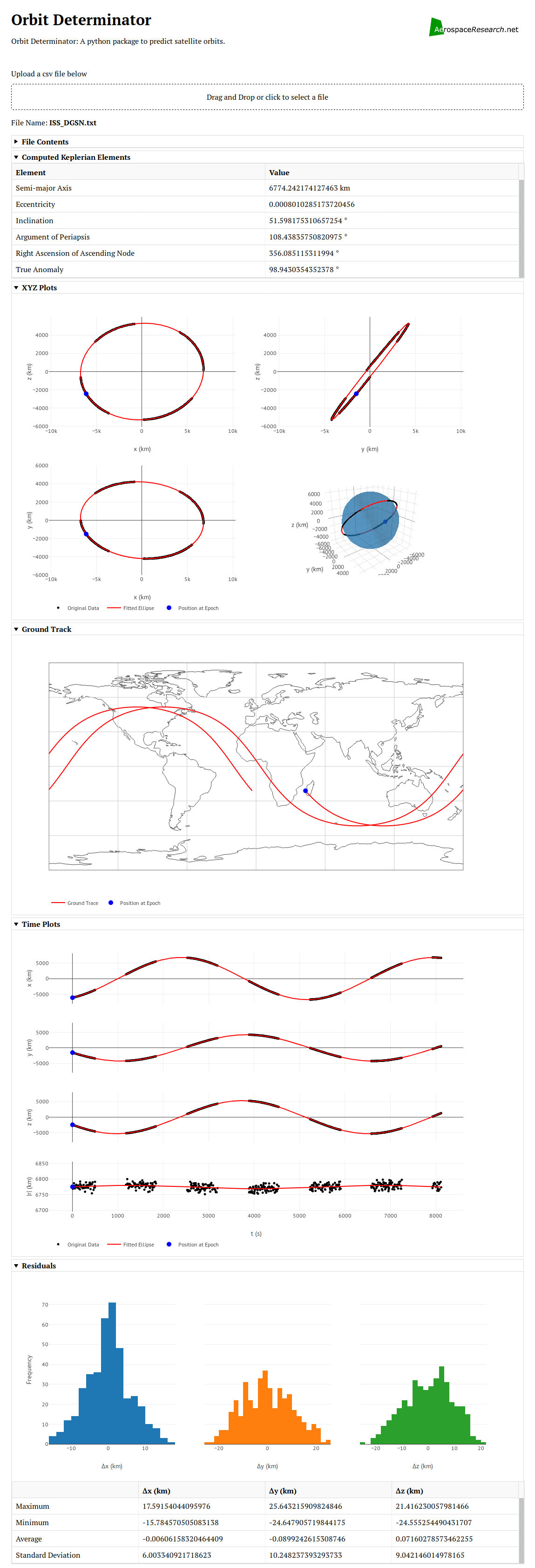Next Steps

In the next couple of weeks, I will be tackling one of the hardest things in my proposal – the Kalman Filter. The Kalman Filter will take predictions from SGP4 and observations from real life/DGSN simulator and combine them to give more precise outputs. To do this first we have to synchronize the two streams of data (model and observations). Then we have to make the actual filter and pass the inputs through it. After that, we have to update the state in such a way that the filter can be used again. That’s a lot of work, so I am looking forward to a very exciting week ahead! 🙂

We got important stuff done in weeks 3 and 4. Everybody knows that visuals and graphics are very important for presentation purposes. The most popular library for plotting is matplotlib. It can generate excellent plots but in the end, they are static images. Instead of static images it’s better if some interactive content is presented. So we decided to make a webapp for OrbitDeterminator. A webapp makes it easier for the end-user to run the program. It can also be hosted on a publicly-accessible server, which means that anyone can use it without going through the pain of downloading and installing the program. For making the webapp, my mentor Alexandros suggested the excellent Dash library by Plotly.

Dash by Plotly

Dash is a Python library that can be used to make web applications. The library is built to be hosted on a server and be used by multiple people at once. It is powered by Plotly which produces beautiful, interactive plots in the browser itself. Programming in Dash is simple. First, you have to define the layout of the app in the form of a list of html components. You can style them as you like or add additional parameters. After this, you have to define callback functions. These functions will be triggered whenever the user interacts with the UI (like pressing a button, or typing some text). These functions can be used to change the elements displayed on the app. This makes the app interactive.

Designing the app

For now, OrbitDeterminator’s primary function is to find a good set of orbital elements that match a noisy set of observations. The webapp will be a graphical way to do this. Observations are stored in CSV files in the following format:

# Comments
# here.
#
# t x y z
<time_1> <x_1> <y_1> <z_1>
<time_2> <x_2> <y_2> <z_2>
...
<time_n> <x_n> <y_n> <z_n>

So the webapp must have a place to upload csv files. We also want to show the name of the file and the file contents in case the user has uploaded the wrong file. And of course, we have to show the results and plots of the results. After discussing with Alexandros, I settled on this layout:

• File upload box
• File name and contents
• Keplerian elements
• Spatial plots
• Ground track
• Coordinate vs time plot
• Residuals plot

But the user might not require all this information at once. So all the components must be collapsible, to hide them from view if not required. Making the webapp required lots of googling but was relatively easy. The end result is this:

All the plots are interactive. You can zoom, pan, and rotate them. You can also save any plot you want as a png file. Most of the plots were straightforward. The most difficult plot was the ground track, whose algorithm I will discuss below.

Plotting the ground track of a satelllite

To plot the ground track, we have to know the position of the satellite with respect to the Earth’s surface. First, I thought that just converting the coordinates into polar form and plotting φ vs θ would do the job. But I forgot that the satellite coordinates were measured with respect to an inertial (fixed) reference frame, whereas the Earth’s surface is rotating. So the actual coordinates will be different. I went through two articles on CelesTrak and Astronomy StackExchange to come up with the algorithm.

NORAD uses True Equator Mean Equinox (TEME) reference frame for its TLEs. In this frame, the origin is at the Earth’s centre. The z-axis points toward the North Pole. The x-axis points to the vernal equinox. And the y-axis completes the right-handed coordinate system.

We need to convert coordinates in TEME to an Earth-Centered-Eath-Fixed (ECEF) reference frame. In such a frame, the origin is at the Earth’s centre and the the coordinate axes are fixed to the Earth’s surface (which means that they rotate along with the Earth). Many such frames exist but the standard one is the International Terrestrial Reference Frame (ITRF). In this frame, the z-axis points toward the North Pole, the x-axis points toward 0°E 0°N. And the y-axis completes the coordinate system. Since both TEME and ITRF share a common z-axis, the latitude will not be affected. Only the longitude will be shifted by a certain amount. This amount, known as the Earth Rotation Angle, is the angle between TEME’s x-axis and ITRF’s x-axis. Now I will write down the pseudocode I used to determine this angle.

Let t be the time at which we want to find the Earth’s rotation. Let t_mid be midnight on the same day, so that t - t_mid is the UTC time during the day. Let J2000 be the time Jan 1 2000 12:00 pm UTC(this is the J200 epoch). Then the pseudocode is:

days_since_J2000 = t_mid - J2000
# multiply the above by an appropriate 
# constant to convert the units into days

# centuries since J2000
Tu = days_since_J2000/36525

# effects of precession of the Earth's axis
tg0h = 24110.54841         +
     8640184.812866 * Tu   +
           0.093104 * Tu^2 -
           6.200e-6 * Tu^3

# Greenwich Mean Siderial Time in seconds
tgt = tg0h + 1.00273790935 * (t-t_mid)

# rotation angle in degrees
rotation_angle = (tgt%86400)*360/86400

After getting the rotation angle, we can subtract it from θ to get the actual longitude.

Putting everything together , we get this plot of the ISS for 21st May 2018 18:27:54 UTC. I used this NASA website to generate the NASA ISS plot.

As you can see, the results line up pretty well. Note that this is a simplified model and is not super-accurate, but it gives roughly the same results.

Future Work

• Integrating the SGP4 model into OrbitDeterminator.
• Making a DGSN simulator (this will be used until the real DGSN starts working).
• Making a Kalman filter to combine the two sources of data.

Hello World!

I have been selected to work for AerospaceResearch.net under the Google Summer of Code program. Since I am a new contributer here, I think I should give a short introduction first. I am Arya Das, an undergraduate student of computer science at Indian Institute of Technology, Patna. I am highly passionate about space. I am also interested in robots, flight simulators, playing piano and swimming.

In this blog post I am going to describe my experience so far at AerospaceResearch.net and the project I am working on.

„[GSoC2018|OrbitDeterminator|Arya] Week #1-2 – Hello World!“ weiterlesen