During these weeks, I worked on coding a high-level interface for two Gauss method applications of orbit determination: Earth satellites and asteroids.
One of the main differences with respect to my previous work, is that we relied heavily on the
astropy library (www.astropy.org), a Python library for astronomical calculations. One of the main factors which inclined us to use this library, is that it has a lot of useful functions, it is relatively well-tested, gives more consistency to the code, and also avoids typos (e.g., in numerical values of astronomical constants). We also incorporated the poliastro library, mainly to use its implementation of the Stumpff functions.Changes in implementation
One of the main changes with respect to the previous version of our implementation, was the abstraction of a „core“ computation of the Gauss method and its refinement iterative stage, regardless of the case being handled, whether it is an Earth-orbiting object (satellite, space debris, etc.) or a Sun-orbiting object (main-belt asteroid, Near-Earth asteroid, comet, etc.). This abstraction is implemented in the
gauss_method_core and gauss_refinement function, which are low level functions and may be adapted for user-defined applications.A new feature of the latest version of the code, is that in case of having multiple solutions to the Gauss polynomial, now the user is able to select distinct roots for each occurrence of the multiple solutions. As we will see in examples below, multiple positive solutions to the Gauss polynomial are common when handling real-world data. In the case of finding more than one feasible solution to the Gauss polynomial, the code spits out all the feasible roots found; this allow the user to select the adequate root to the polynomial.
Also, the execution speed was improved for the Near-Earth asteroids case: when handling multiple observations, instead of reading the MPC-formatted file each time and retrieving the relevant triplet of observations, now the file is read only once. Since the observation files from MPC are typically a few thousand lines long, this improved the execution speeds about 10x.
Another important change, is that now the local mean sidereal time is computed using
astropy ’s sidereal_time method for SkyCoord objects instead of using our own implementation. While doing this, we were able to identify a bug in our implementation of the computation of the local sidereal time!Finally, in the case of Sun-orbiting bodies, the average orbital elements are computed in the heliocentric J2000.0 ecliptic frame; this allows us to directly compare our results, for example, with the orbital elements listed in the JPL’s Horizons online ephemeris service.
Example 1: Ceres
The code needed to run this example may be found in the
gauss_example_ceres.py in the orbitdeterminator/kep_determination folder. There, a high-level interface for processing of multiple observations of MPC-formatted files is used in order to compute a preliminary orbit for Ceres, using 27 observations of this body. The example may be run from the command line simply by doing $ python gauss_example_ceres.py. The only caveat is that, as stated in the previous blog post, the computation relies on using the NASA-JPL DE 430 ephemeris for the Earth and the Sun in SPK format, so in order to run this example the de430t.bsp file must be present in the kep_determination folder. This file may be found at ssd.jpl.nasa.gov/pub/eph/planets/bsp/de430t.bsp and may be downloaded via FTP. We decided against uploading this file to the orbitdeterminator repo, since it’s around 100MB in size.After running a few preliminary code, the example calls the
gauss_method_mpc function, which takes 27 ra/dec observations in total, separated by time intervals of around 1 month, in order to compute the orbit of Ceres. That is, this function read the whole MPC file for Ceres, reads from it only 27 lines, and from it then computes the Ceres orbit using the Gauss method taking three by three observations. We noticed that, if shorter intervals were taken, then the Gauss method showed some convergence problems. We also found that these problems with very short observational arcs for the Gauss method have been described, e.g., in [1].Below, we show the output from the
gauss_method_mpc function. There, the Sun is shown as a yellow dot at the center of the plot. The computed orbit of Ceres is shown in red along with the estimated states using the Gauss method. Also, in blue, the orbit of the Earth is shown.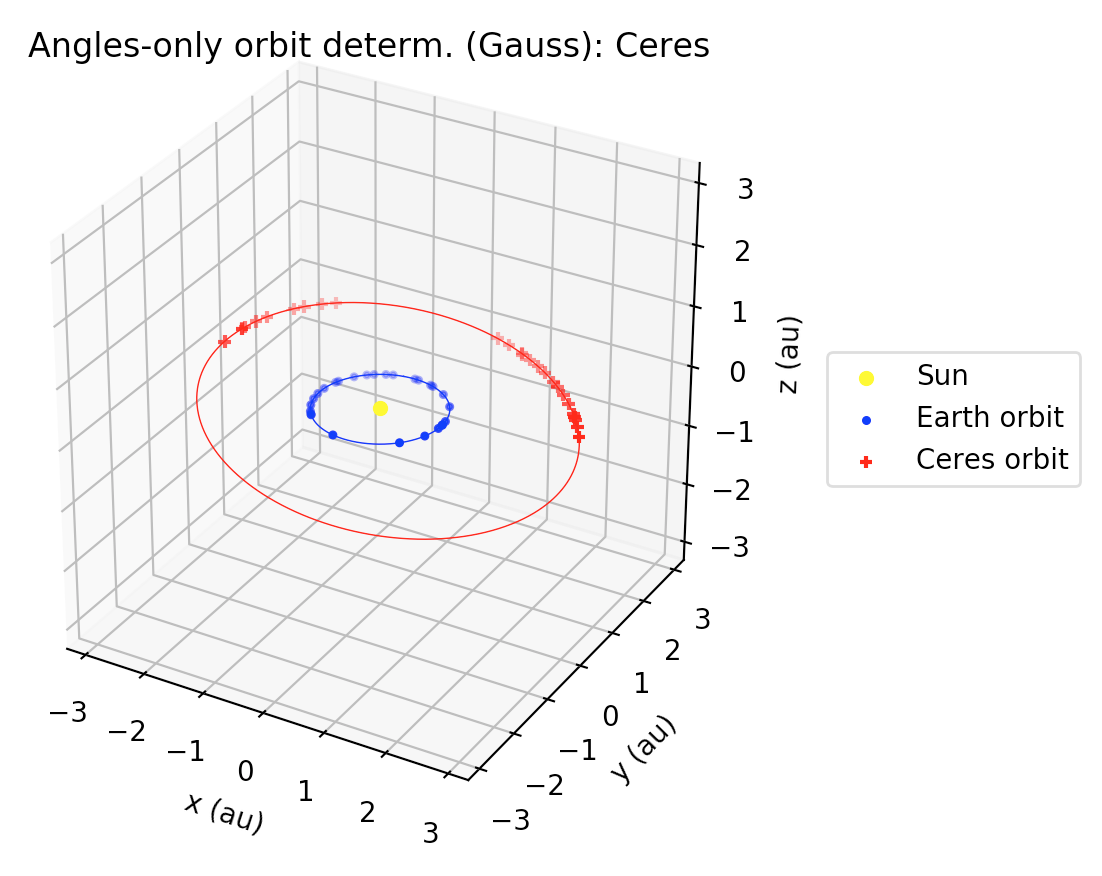
The heliocentric ecliptic average orbital elements (we use
astropy’s value for the mean J2000.0 obliquity of the ecliptic), are:a = 2.768129232786505 au
e = 0.07938073212954426
I = 10.584725369990045 deg
Ω = 80.4066281982582 deg
ω = 73.07336134446685 deg
On the other hand, the heliocentric ecliptic orbital elements reported by NASA-JPL in Horizons are:
a = 2.767218108003098 au
e = 0.07610292126891821
I = 10.60069567603618 deg
Ω = 80.65851514365535 deg
ω = 71.44921526124109 deg
Thus, we see that although some differences exist, our results give a very good first approximation to the orbit of Ceres, using only 27 observations! Indeed, Gauss method is really powerful!
Example 2: Eros
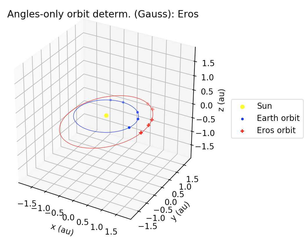
In this example we compute the orbit of the first-ever discovered Near-Earth asteroid: 433 Eros. Here, we use the Gauss method with only 4 ra/dec observations.
For the heliocentric ecliptic orbital elements, we got the following results:
a = 1.4900359723265548 au
e = 0.2222907524713779
I = 10.87373869230558 deg
Ω = 303.89500826351457 deg
ω = 175.09494980703403
JPL Horizons online service tells us, on the other hand, that:
a = 1.458251585462893 au
e = 0.2229072630918923
I = 10.82944790594134 deg
Ω = 304.4109222194975 deg
ω = 178.6283758645153 deg
Again, although we observe some small differences, the results we have are pretty close to the ones computed by JPL. And now, we used only 4 observations!
References
[1] Milani, A., Gronchi, G. F., Vitturi, M. D. M., & Knežević, Z. (2004). Orbit determination with very short arcs. I admissible regions. Celestial Mechanics and Dynamical Astronomy, 90(1-2), 57-85.