GSoC2021: Development of an FDIR algorithm using Neural networks

The goal of this project is to develop a failure detection, isolation and recovery algorithm (FDIR) for a cubesat, but using machine learning and neural networks instead of the more traditional methods.

Motivation: What is an FDIR algorithm and why is it usefull?

One of the most challenging parts of space missions is knowing and controlling where your spacecraft is, what is its relative orientation with respect to earth and how it is moving. Being aware of these three things is crucial to know if your spacecraft is flying too high or too low, too close to other spacecrafts, or simply if its oriented in a way that will allow it expose its solar panels to the sun to produce power or to point its antenna down to earth for calling home.

To perform this crucial task of computing and controlling its position and orientation spacecraft are designed with a variety of sensors and actuators that, together with proper control algorithms, ensure that your satellite remains where you want it and pointing in the right direction. This is often referred to as Attitude and Orbit control subsystem or AOCS.

Since this subsystem is critical for the spacecraft, it is needless to say that a failure in one of these sensors or actuators could easily kill your spacecraft and put and end to your mission. A faulty reading of a gyroscope that says that your spacecraft is rotating when it is not, a dead gyroscope that gives no signal and can’t tell if it is, or just a faulty thruster that provided more thrust than it should could leave your spacecraft spinning uncontrolled.

For these reason, providing the spacecraft on board software with a way of detecting these kind of failures as well as guidelines on how to proceed if one of these failures is detected is crucial for any space mission. This is done by means of the so called Failure Detection, Isolation and Recovery algorithms (FDIR).

Traditionally, these types of algorithms where simple, as they where based mainly on hardware redundancy , i.e., having many sensors that measure the same thing so that if one fails, you could detect the failure by looking at the rest and seeing that the signal is not consistent, isolate the failure by ignoring the reading from that sensor, and recover from the failure simply by continue to listen to the rest non-faulty sensors. While this is a valid and robust strategy to FDIR, it requires hardware redundancy of many spacecraft sensors and actuators, which means carrying on board more gyroscopes or reaction wheels than you actually need.

In recent years however, there has been a rising interest in low-cost space platforms such as Cubesats, pico or nano satellites that perform missions with much smaller budgets. One of the strategies used in these missions to reduce costs is to replace hardware based functionalities by software based ones, reducing therefore the number of components on board, the weight and power demands and overall complexity.

Replacing a hardware redundancy based FDIR strategy with a software based strategy is a perfect example of this. If your on board computer is capable of detecting a drift or a bias in the measurement of a sensor and correcting it without the need of comparing it with redundant sensors, or comparing it with the smallest number of redundant sensors possible then your mission might still be capable of safe operation, but minimizing the weight, power and cost penalties of hardware redundancy. There many ways to perform FDIR algorithms that focus on software instead of hardware, in order to explore some of the less conventional ones, it was decided to focus the project around machine learning and neural networks.

Project description

The goal of the project was then to set the basis of a neural network that could work to detect possible faulty signals from a cubestas sensors and actuators during its operation. This project had then two distinct lines of work:

  1. To develop or modify an existing simulator of a Cubesat to generate and extract the data from the sensors and actuators. This data is needed to train and test the Neural Network.
  2. To create an script capable reading and preprocessing the data from the simulator as well as creating, training and testing the neural network.

For the first, task an existing Cubesat simulator that included its own FDIR algorithm was used. This simulator written by Javier Sanz Lobo using Simulink included among its features the ability to simulate not only the cubesats motion, but also the readings from gyroscopes, reaction wheels and thrusters, as well as the capacity to induce artificial failures on the different components during the simulation. The original simulator can be found linked in the following repository:

https://github.com/msanrivo/SmallSat_FDIR

Several modifications where made to this simulator in order to fit it to it’s desired purpose. Among these it is worth highlihting:

  • The ability to Change the initial conditions to randomly generated ones within a desired range
  • A Matlab code that ran the simulator in a loop with random failure scenarios to generate the training and testing data
  • The capacity to export the readings from the sensors and actuators during the simulation to .txt files with the desired format.
  • Disabling the FDIR algorithm so that the simulated readings of the artificial failures remained unchanged.
  • The capacity of failures to occur at different times rather than at the start of the simulation.

For the second line of work, a scrip was written from scratch in python 3.8 using keras from the TensorFlow library to build, train and test the neural network. At the day of publishing this post, there are currently two scripts that read the data from 6 gyroscopes and 4 reaction wheels of the cubesat in the simulator and use one thousand simulations to train a Neural Network and a convolutional neural network. In both cases the network is then tested with another one hundred simulations to evaluate its real accuracy.

The end result is two types of neural networks that are both capable of predicting not only the most likely failure scenario that corresponds to that data, but also the probability of each individual failure scenario, which is a valuable input for future steps in the process of developing a fully functional FDIR algorithm.

Results

Currently both the traditional neural network and the convolutional one achieve accuracy values of around 70% in their predictions. Note that with 6 gyros and 4 Reaction wheels and the limitation of a maximum of two gyros and two reaction wheels failing the number of possible scenarios rises up to 242, which makes it hard to perform predictions.

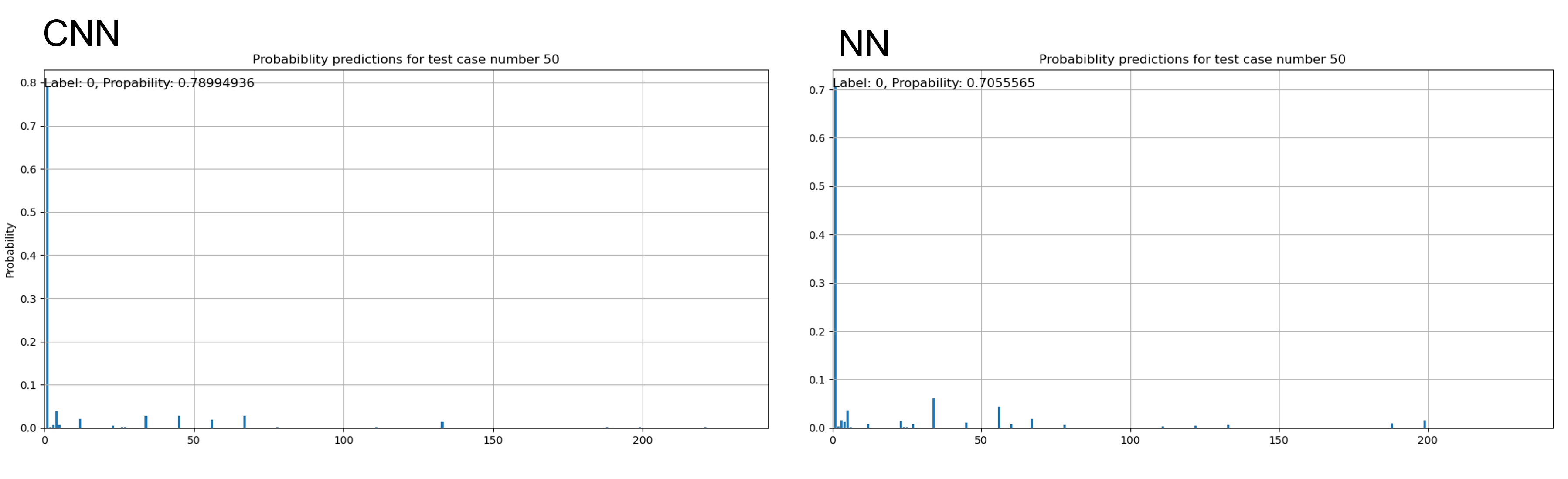
Simpler scenarios where none of the devices fail are easily identified by both networks, as is the case of the following figure where both predict the correct outcome with a probability higher than 70%:

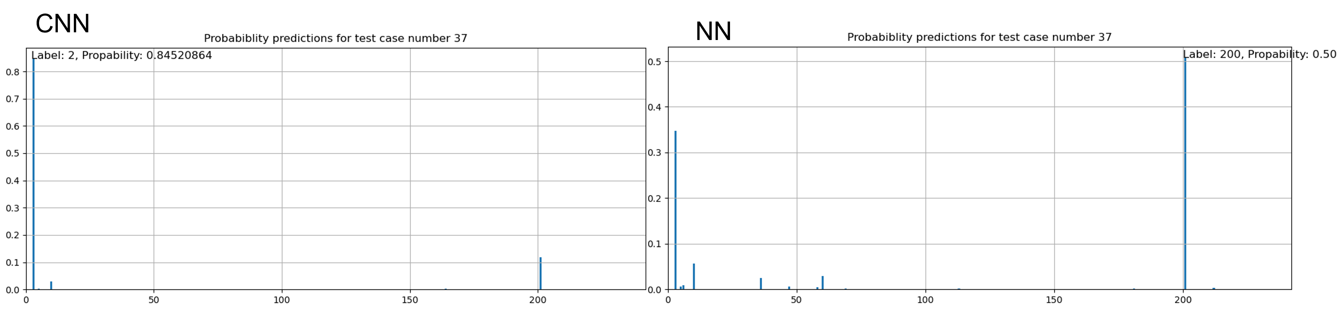
More complex scenarios where one or several devices fail reduce this prediction probability, making them capable of predicting correctly the failure of one device, but rarely all of them. In this cases, however, usefull information is provided by the probabilities, as the correct scenario can be found among those with the highest probabilities even if it is not the one with the highest.

Take for example the case depicted in the following figure where only one reaction wheel fails. The CNN is capable of predicting the correct scenario, but the NN predicts a scenario in which not only the aforementioned wheel fails, but also two complementary gyros as well. Note that even when predicting the wrong scenario, the NN shows the correct one as the second most likely.

Future work

A lot has been achieved during this GSoC period, yet there is still plenty of work ahead in this ambitious project. Among the features that are still to be implemented and tasks to be performed there are:

  • Continue to improve the neural networks to achieve better results at higher computational efficiencies.
  • Improve the simulator to generate better failure scenarios for thrusters.
  • Expand the FDIR capabilities of the network to include the simulated values of thrusters.
  • Research on reducing the number of input arguments to reduce the order of the problem and increase efficiency.
  • An interface between simulator and neural network to test and simulate in parallel.

Useful links

Github Repository: https://github.com/Rafabadell/FDIR_Neural_Networks

Author e-mail: Rafael.Badell@aerospaceresearch.net 

[GSoC2021] CalibrateSDR GSM Support

Overview

CalibrateSDR developed by Andreas Hornig, is a tool developed to determine the frequency drift of Software Defined Radios precisely using sync pulses of various Signal Standards.  

Cheaper SDRs use a low-quality crystal oscillator which usually has a large offset from the ideal frequency. Furthermore, that frequency offset will change as the dongle warms up or as the ambient temperature changes. The result is that any signals received will not be at the correct frequency, and they would drift as the temperature changes. CalibrateSDR can be used with almost any SDR to determine the frequency offset.

The work on GSM (2G) has been done by Jayaraj J, mentored by Andreas Hornig, as part of Google Summer of Code 2021, the working directory for the same can be found at Github.

proposed working of CalibrateSDR – made GSM signal compatible (the below guide shows how to get started)

Project Description

GSM uses time division to share a frequency channel among users. Each frequency is divided into blocks of time that are known as time-slots. 8 time-slots are numbers TS0 – TS7. Each time slot lasts about 576.9  μs. The bit rate is 270.833 kb/s, a total of 156.25 bits can be transmitted in each slot.

Each slot allocates 8.25 of its „bits time“ as guard-time, split between the beginning and the end of each time slot. Data transmitted within each time slot is called a burst. There are several types of bursts.

Frequency correction burst is a burst of a pure frequency tone at 1/4th the bitrate of GSM or (1625000 / 6) / 4 = 67708.3 Hz. By searching a channel for this pure tone, we can determine its clock offset by determining how far away from 67708.3Hz the received frequency is.

How is it working?
  1. Scanning of GSM Channels is based on the ARFCN frequency bands. For tuning into GSM Frequency, the ARFCN script can be used. We give the input of band to scan, the result will be the frequency. If we input the „scan all“ option, it will scan the whole GSM Frequencies in the given band and return the offset calculated from each frequencies. The code for the same can be found at: https://github.com/aerospaceresearch/CalibrateSDR/blob/jyrj_dev/calibratesdr/gsm/arfcn_freq.py
  2. After scanning channels in specific bands using ARFCN, the program will record the sample in the given sample rate. Make sure the SDR is connected with the device, or we can record it and give the input as a wave file.
  3. The determination of the position of FCCH bursts that we receive in SDRs is done by the code in fcch_ossfet.py. We measure it by how much shifted is the FCCH burst, than what we expect, that is at 67708.3 Hz from the frequency centre. Simply, if no offset is there, we could see these tone bursts at 67708.3 Hz offset concerning the centre frequency of the channel.
  4. The final output we receive include
    • Frequency drift from the expected FCCH position
    • The Offset of SDR in PPM
  5. The whole code works from the main cali.py and inturns gsm.py files
To test with the IQ_file.wave:

After cloning the repo locally, run the setup to install the requirements using the command: python setup.py install

After that, to run the visualization plots, run:

python cali.py -m gsm -f <location of wav file> -rs <sampling rate> -fc <frequency center>

First, we will get the plot of the average power spectrum plot. Play with the code to increase the N value, and you can see the sharpness of the line.

Further plots generated includes TDMA frames, the position of FCCH bursts visualisation as given below.

Screenshot-spectrogram_hann-Zoomed.png

We can see the pure tone FCCH bursts are occurring at specific intervals and can be visualized as small blue dots at a range of 0.25 from the centre.

Thus implementation of a filter bank and calculating the positions of these FCCH bursts will give us the offset frequency since we know these FCCH bursts occur at a distance of 67708.3 Hz from the frequency centre.

The average power spectrum of Discrete Fourier Transforms

Usage

Test files for GSM, recorded by Andreas can be found here.

  • Setup the environment, make sure the requirements are installed (preferably in a virtualenv). Use the setup.py to install necessary requirements.
  • To view the parameters for input run ~$ python cali.py -h

usage: cali.py [-h] [-f F] [-m {dab,dvbt,gsm}] [-s {rtlsdr}] [-c C] [-rs RS] [-rg RG] [-rd RD] [-nsec NSEC] [-gr] [-v] [-fc FC]

optional arguments:
-h, –help show this help message and exit
-f F select path to input file
-m {dab,dvbt,gsm} select mode
-s {rtlsdr} scan with rtlsdr
-c C scan by „all“ channels, by channel number „0,1,…n“ or by block name
-rs RS file/scan sample rate
-rg RG scan with gain
-rd RD scan with the device
-nsec NSEC scan for n-seconds
-gr, –graph activate graphs
-v, –verbose an optional argument
-fc FC frequency centreSetup the environment, make sure the requirements are installed (preferably in a virtualenv). Use the setup.py to install necessary requirements.

  • If testing with a recorded wav file, enter the parameters as:
~$ python cali.py -m gsm -f <location of wav file> -rs <sampling rate> -fc <frequency center>
  • If testing with an SDR stick, specify the ARFCN band, or specific frequency centre to scan for the GSM channel.

The ARFCN Bands include: GSM_850, GSM_R_900, GSM_900, GSM_E_900, DCS_1800, PCS_1900. For more information about the arfcn, checkout here.

Example usage:

~$ python cali.py -m gsm -s rtlsdr -c 900

The above parameters can be changed according to user needs. -rs can be specified with sample rate. The exact sample rate will be shown with the result. Make sure the SDR is connected when running the code with -s rtlsdr argument. Specify the -fc frequency argument, if the scan is to be done with a single frequency.

The expected output would look like this:

{'f': None, 'm': 'gsm', 's': 'rtlsdr', 'c': '900', 'rs': 2048000, 'rg': 20, 'rd': 0, 'nsec': 10, 'graph': False, 'verbose': False, 'fc': None}
let's find your SDR's oscillator precision
scanning…
starting mode: gsm
Found Rafael Micro R820T/2 tuner
Exact sample rate is: 270833.002142 Hz
Scanning all GSM frequencies in band: GSM_900
Offset Frequency: 31031.66666666667
Offset in PPM: 33.179448397684716

The Offset calculated from the frequency drift between fcch positions can be precisely derived and can be used to correct the oscillator.

Potential further improvements:
  1. LTE Signal support need to be included (currently in focus), and much more standards need to be made compatible for a wide usage of the tool.
  2. Making a platform-neutral API to communicate with more SDR devices.
  3. Optimising the user interface (command-line tool can be made more user friendly).

References:

Find out the project updates in my branch and do give a star for the project in AerospaceResearch org:

https://github.com/aerospaceresearch/CalibrateSDR/tree/jyrj_dev

[GSoC2021] CalibrateSDR GSM Support – first coding period

Introduction

CalibrateSDR developed by Andreas Hornig is working perfectly with signals DAB+. We can use the python program to calibrate SDR devices. As part of the Google Summer of Code, I have been working around GSM Signal Standard to make CalibrateSDR compatible with it.

Before moving on, please read the initial blog on using CalibrateSDR, written by our mentor. The primary focus of this project is to extend the applicability towards more signal standards, so as to make it helpful for the SDR community. As DAB+ is mainly used in Europe, Signal standards like GSM, LTE, NOAA-Weather Satellites (use their sync pulses within the data) can be used.

Currently, it uses the pyrtlsdr package, which makes it work with RTL-SDR. Piping the API to work with other SDRs will also make the project have a wide range of applications in the SDR Community.

My first weeks of coding relied generally on implementing GSM signals. Working with the GSM frequency correction channel to calculate the offset is my primary task.

Proposed final working of CalibrateSDR

Working of GSM to calibrate the SDRs

GSM uses time division to share a frequency channel among users. Each frequency is divided into blocks of time that are known as time-slots. There are 8 time-slots that are numbers TS0 – TS7. Each time slot lasts about 576.9  μs. The bit rate is 270.833 kb/s, a total of 156.25 bits can be transmitted in each slot.

Each slot allocates 8.25 of its „bits time“ as guard-time, split between the beginning and the end of each time slot. Data transmitted within each time slot is called a burst. There are several types of bursts.

„Frequency correction“ burst, which is a burst of a pure frequency tone at 1/4th the bitrate of GSM or (1625000 / 6) / 4 = 67708.3 Hz. By searching a channel for this pure tone, we can determine its clock offset by determining how far away from 67708.3Hz the received frequency is.

How is it working?

A more robust way is to implement a hybrid of the FFT and filter methods. We could use the adaptive filter as described in the paper: G. Narendra Varma, Usha Sahu, G. Prabhu Charan, Robust Frequency Burst Detection Algorithm for GSM/GPRS (https://ieeexplore.ieee.org/document/1404796)

After finding the position of FCCH bursts that we receive in SDRs, it will be easy to calculate the offset. We measure it by how much shifted is the FCCH burst, than what we expect, that is at 67708.3 Hz from the frequency centre. Simply, if no offset is there, we could see these tone bursts at 67708.3 Hz offset with respect to the centre frequency of the channel.

I have completed the program to output the channel frequencies from the given ARFCN numbers of GSM. Check the code for the same here.

Detect and visualize the FCCH bursts!


Currently, the program has been tested only with IQ Wav file recordings. Even though the code has been designed to work with RTLSDR sticks, it is not tested yet with a live connection. Find the link to test files here.

After cloning the repo locally, run the setup to install the requirements using the command: python setup.py install

To test with GSM files, run:

python cali.py -m gsm -f <location of wav file> -rs <sampling rate> -fc <frequency center>

First, we will get the plot of the average power spectrum plot. Play with the code to increase the N value, and you can see the sharpness of the line.

The figure above shows the TDMA frames generated by the GSM Signal.

To determine the FCCH bursts from the signal, plot the spectrogram, using the function present in gsm.py. The spectrogram_plot function will do the fft and outputs the figure.

The generated FCCH bursts detection can be visualized as shown below:

We can see the pure tone FCCH bursts are occurring at specific intervals and can be visualized as small blue dots at a range of 0.25 from the centre.

Thus implementation of a filter bank and calculating the positions of these FCCH bursts will give us the offset frequency since we know these FCCH bursts occur at a distance of 67708.3 Hz from the frequency centre.

Will update the code after testing with gsm channels, and the function to calculate the final frequency offset will be committed to the repo.

The workarounds for the second coding period are implementation of LTE and NWS as well as the bridging of a more generalised SDR API, SoapySDR API, which has Python bindings to use as well.

Find out the project updates in my branch here: https://github.com/aerospaceresearch/CalibrateSDR/tree/jyrj_dev

References:

[GSoC 2020 | MOLTO | Brandon] Refactorization MOLTO

Introduction

Hi, my name is Brandon Escamilla, I am an Aerospace Engineer by Universidad Marista de Guadalajara (Guadalajara, México). This is the second time I got selected for the GSoC. I am really grateful for this opportunity. This time, I came along with a proposal to improve the actual MOLTO project. The same I did work the last year. MOLTO is a big project, which has tons of work before going to production. Last year, I worked in a way to connect MOLTO with a user interface, it was not an easy work since MOLTO is a Matlab tool which requires special connections and is not as easy as consuming a normal API, so I did create an API with Python/Flask to communicate my requests from the Frontend to Matlab directly. It did work, we did communicate successfully with the Matlab tool. But there were some problems we need to resolve in order to have a „production environment“. At the end of the GSoC, we had a UI created in React.js, an API using Flask, and a local database using SQLite. This was enough to prove the architecture I wrote in my proposal, easy architecture to get to the web those projects created in Matlab which can’t go to production because Matlab closed license.

Last year blog: [GSoC 19′ |UC3M ] MOLTO – Mission Designer]

So, here you have the new flow of MOLTO from a route-based perspective, and from a logical flow.

The main issues that needed to be solved before to go to production were the ones I will list below:

  1. Error communication between Matlab and Python.
  2. Delete Real-time communication between UI – Python – Matlab. (Sockets)
  3. Create a new service based on Codes to retrieve the mission.

But there were also some improvements needed to be added with lower priority:

  1. Friendly user interface for new users.
  2. New Design
  3. Create a database in production to save missions configuration and results.
  4. Create an email service to send mission codes.
  5. Create CMS to add information in an easy way for maintainers.
  6. New view for the service based on codes.
  7. Improve deployment of Frontend.
  8. Response optimization from Matlab Genetic Algorithm.
  9. Toy problem for new users.
  10. Optimize responsive views of the site.
  11. Improve Celery implementation for Background tasks.

Before continuing, I would like to add that after GSoC, I continued working on MOLTO, adding small features, and improving user experience as fas as I could. In our constant communication between my last mentor David and I, he did invite me to start a research stay in the University Carlos III where he was doing his Doctorate. This led to another experience where David has been my bachelor’s degree thesis advisor. (A good story thanks to GSoC! ?)

Hands-On!

Once accepted, I started working on my proposal which did look something like this:

1. CMS Implementation

For this purpose, I did use an open-source application called Strapi, which allows you to develop a CMS locally and in production in an easy way. It helps you to develop the database, API, endpoints, CDN requests, models, emails, and more…

I did install Strapi locally and started creating the services were needed for MOLTO which can be divided in this way:

  1. Collaborators
  2. Missions
  3. Users
  4. Email Service
  5. Motors

Once I create all the services described before, I just started to launch the CMS to production. The easiest way to do this is using Heroku, which allows you to have an app in production with very few steps and configuration. Finally, you can find the Admin in this URL: https://molto-admin.herokuapp.com/admin, Of course, it has a login and just the maintainers of MOLTO can access. But I leave you a few screenshots, so you can see the interface.

I am using a PostgreSQL database which actually is a plugin from Heroku app. ✅

And this is the documentation of the endpoints:

https://molto-admin.herokuapp.com/documentation/v1.0.0

2. New design MOLTO

Before going to production we needed a new design because the first one was more like an MVP, finally, I added a link to the old site, the designs, and the newly implemented design. Almost all the components of the website did change, from the home to MOLTO-IT, and also new views were added.

Here I will leave you some screenshots of the old design and the new design. (I will include the links in case you want to check it out )

New site: https://molto-it-ui-old.vercel.app/

New site: https://molto-it-ui.vercel.app/

Another new feature is in the motors section of MOLTO-IT, where you can actually see the motor configuration clicking in more information.

Another feature is the mobile version of MOLTO and the new menu, at this moment is really important to have a good mobile version of websites, since most users will visit your site from their cellphones. So, I did refactor the mobile version and right now is good to work from cellphones.

3. Tour MOLTO

In order to have a better experience in MOLTO, I did try a lot of ways to do it. I started using a library called React tour, and after another one called React joyride, but I did notice that those were very intrusive with the user experience and that actually the performance of the application was really bad when using both libraries. So I did prefer to create my own component which shows an information icon and if you hover on desktop or click it in mobile, display a box with useful information in order to know what to add in the inputs or what are the inputs for.

I found this way less intrusive and useful in my opinion. Here you have one screenshot of this component.

4. New service for creating a mission or search for a mission created.

One of the requirements of the last year was to create a UI with the possibility to see how the genetic algorithm evolves in the time. This was possible, but also a bad idea from a user perspective. Once they select their configuration, they needed to be waiting for the response of the API, this time could go from 3 minutes to 10 minutes – more generations, more population, more time-, which is the time Matlab started the genetic algorithm, in this point Flask opened a socket to start consuming the files were being created in real-time in a directory of the server where MOLTO lives. This was working well but just in one situation: A mission with really low generations and population, since this kind of missions will return results fast. So, once you started a mission with more than 30 generations and more than 50 population, you needed to wait a lot of time before the sockets could return the first generation, and this leads to another problem if the user wanted to see the final generation, the user needed to wait from minutes to hours, without closing the browsers – once you closed the browser, the socket connection finished-. So in the meantime between GSoC and GSoC, I created a new architecture based on codes where you create your mission and the website returns you a code, and also the possibility to send the code to your email, so you could return, in 1 hour, 1 day or 1 week, and all your results will be there stored in the database. Of course, this was a lot of work, I need to almost change most of the logical code was created to connect with Python via sockets. And also new views needed to be created to retrieve the mission, send the code to email, etc.

Almost in the middle of the second evaluation I start working on this, and after days of coding, the new service was available, here I will add few screenshots, but of course, you could to the MOLTO website.

The view which looks for missions, has an input where you need to put the code MOLTO gives you when you finished the configuration of your mission, this input has the ability to detect invalid codes, and also returns the current status of the mission. This is thanks to Celery, which is a tool that before was just running tasks in the background, but with the proper configuration, you can check the status of the mission in real-time. ?

4. Celery and Matlab Errors

As I said at the top of this post, one big problem was that I had issues trying to connect Matlab errors with python, due to this once a mission failed, I didn’t know the real reason why it was failing. At the start, it was not a problem, because I was using always the same JSON for creating missions and testing. But once you put different configurations, it was randomly working, sometimes it works, sometimes it just crashes, and I didn’t know what was happening. So, this year, I decided to solve this issue, as said before, using Celery properly, and also the Matlab Engine For Python.

The big issue was that I was not adding some configurations to check the tasks in the UI of Celery called flower, and I was also not using some configuration to read logs from Matlab in python, It was a hard task, but finally, it is working, so I will put here one screenshot of the logs I am receiving in the server where I can know exactly why Matlab is not working.

I can also see all the missions in real-time in a dashboard, all the missions that failed, all the successful missions, and also the tasks that are running.

5. New host for Frontend

There are a lot of ways to host your frontend applications, we can host our frontend in the MOLTO server, or maybe in another service like AWS, etc. But I recently started using Vercel to host other projects, and it was a great experience since you can have multiple environments for testing, production, development, etc. All of this in one place, connected to your repository in Github or to your CLI. It makes easier the development and that’s why it is the platform MOLTO will be using for frontend hosting.

We have right now two environments dev, and production, all the changes that will be applied to the UI of MOLTO will pass first by dev, after approval all these changes could be applied to production.

6. Toy problem

One problem I faced when I was demonstrating MOLTO was that I was the only person who knows how to use it. That was a problem because you can’t deploy an application to production if it is not intuitive.

In order to improve this situation, I used the based architecture of data management called Redux to pre-load a problem, so every time you enter to MOLTO-IT you can change just the name and go to the last tab, click send, and here you have a useful mission, from Earth to Jupyter. So you can test this mission, and actually see the Pareto front without any problem.

7. New flow with code – Pareto Front

I’ve been talking about the new flow but I didn’t show you how it looks after you put a code that has a finished state. Well, actually, this view has some improvements also.

The first one is that you are able to see all the results from generation 1 to the last generation with its respective results. So you can test any value to plot the orbit. You can also see in real-time how the chart changes once you select another Pareto point.

Conclusion

It was an honor to work again in the Google Summer of Code 2020, finally, I would say I finished what I proposed at the start of this project. I also want to thank all the persons who make this possible, Dr. Manuel Sanjurjo, Dr. David Morante for guiding me, and helping me every time I have issues or problems to resolve. I also want to thank you for the research stay at UC3M, I hope I can continue working along with both in this and other projects.

I also want to thank Andreas Hornig for being there for any question and always provide the necessary stuff to keep working. Also for always remember me the deadlines ?, and pushing me to give the best of me.

As far as I know, this is the last GSoC in which I can contribute as a student ☹️, but my next goal is to keep contributing to open-source and why not contribute also as a mentor if possible in the next GSoC’s. I would really like to share all that I’ve learned during these 2 years. ?

Thank you for reading.

Brandon Escamilla

Useful resources:

  1. Production website: molto-it-ui.vercel.app
  2. Repository: https://github.com/uc3m-aerospace/MOLTO-IT
  3. Email: brandon.escamilla@outlook.com | brandon.escamilla@aerospaceresearch.net