This week I worked on propagating the satellite state. The NORAD TLEs are supposed to be used with the SGP4 propagator. It takes care of major perturbations like the oblateness of the Earth and atmospheric drag. Right now, Aakash is working on making one for our organization. But until then, I decided to work with the SGP4 module by Brandon Rhodes.
Working with SGP4
To make the code, I thought in reverse. We wanted to propagate a state vector from one time to another. So our function should look like this:
def propagate_state(r,v,t1,t2)
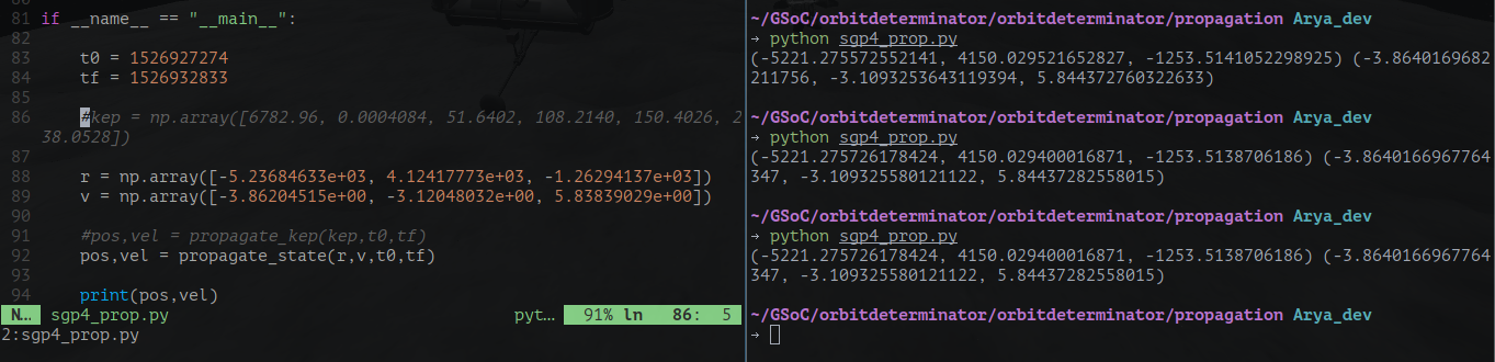
I checked and saw that the module only accepts TLEs as input. So we have to convert r,v to keplerian elements. Then artificially generate a TLE and input it to the module. The Celestrak website specifically asks us not to do this. But when data is not available, one must make approximations. I followed this approach and made the function successfully. However, I wasn’t satisfied. Artificially generating TLEs (which are strings) is computationally expensive. I wanted a direct way to feed the input. So I studied the source code and made another function that does the job without resorting to strings.
To propagate the state, we need to set the following parameters:
whichconst, afspc_mode,
inclo, nodeo, ecco, argpo, mo, no,
satnum, ndot, nddot, bstar,
epochyr, epochdays, jdsatepoch, epoch
The first line has constants which have default values. whichconst is the gravity model which is wgs72 by default. And afspc_mode is False unless you are dealing with old TLEs.
The second line has paramters that can be set directly from keplerian elements. The elements in order are inclination, longitude of ascending node, eccentricity, argument of periapsis, mean anomaly and number of orbits in a day.
The third line has parameters which are available in TLEs but they are not available to us. I set satnum, ndot and nddot to 0. satnum is irrelevant for the calculation. And ndot and nddot are normally very close to 0. For the bstar term, I couldn’t set it to zero because that would disable drag simulation. So I went through the b* terms of many satellites and got an average value of b* = 0.21109x10⁻⁴. Unless a b* term is supplied, this is used for the simulation.
The last line has parameters related to the epoch. These paramters in order are epoch year, day of year, julian date of epoch, and a Python datetime object of the epoch. These can be set by converting the epoch into a datetime object and manipulating it.
After putting together all this, you get the propagator:
The DGSN Simulator
Until the real DGSN comes online, we must work with a simulator. A live simulator will also allow us to make live predictions of the satellite. I thought that just running the propagator in an infinite loop will do the job. But it turned out to be more difficult. In a real time infinite loop, I can’t pause to take input. So I can’t control it while it’s running (like stopping or resuming it). Therefore I resorted to multi-threading. The main thread is used for controlling the program and calculations are done on another thread.
First, I made a basic simulator. It just prints the current location of any satellite, given it’s state at some previous time. There is a speed setting for development purposes too. The demo below is printing the position of the ISS every second in cartesian coordinates.
Next step was to add noise and gaps. Gaps are periods when no signal is available from the satellite. Adding noise was very easy. A random value between -15 and 15 kms is added to every component of the position vector. To add randomness in time, the time period between each observation is randomly decided. Implementing gaps was tougher.
I thought about it and deduced that gaps will be caused when the antenna can’t see the satellite. This will be caused by the rotation of the Earth and the revolution of the satellite. So the gaps will be periodic with time. To implement this, I wrote the following algorithm:
omega = <frequency>

p = abs(sin(omega * t))
if (p >= <threshold>):
    # process the output
    # as if the satellite is
    # within range
else:
    # continue as if the satellite
    # is out of range
The figure below shows the working of this algorithm:
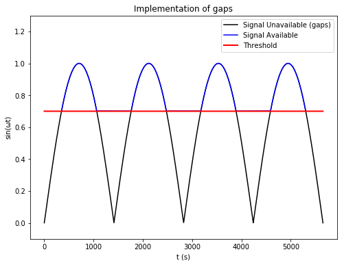 By changing
 omega, one can control the frequency of the gaps. By changing threshold, one can control the duration of the gaps. A lower threshold means smaller gaps and vice-versa.
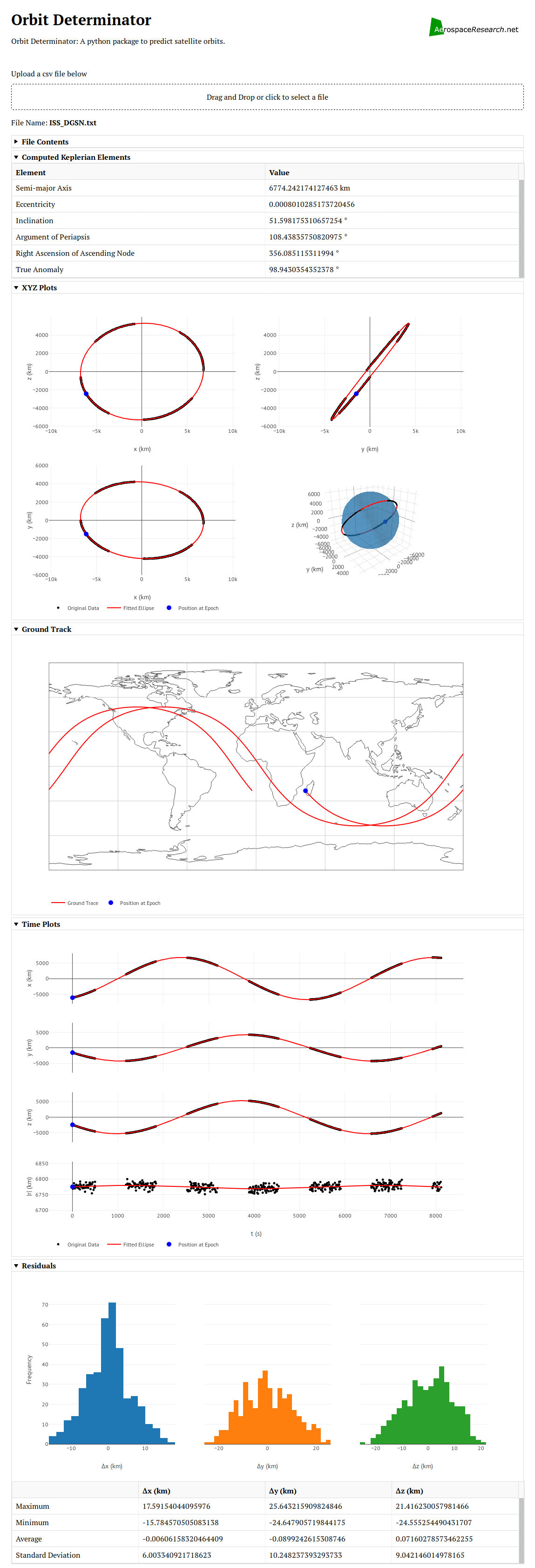
Putting it all together, I ran the simulator for 2 full orbits and plotted the results on the webapp I made last week. The results look pretty satisfying. 🙂
 Next Steps
In the next couple of weeks, I will be tackling one of the hardest things in my proposal – the Kalman Filter. The Kalman Filter will take predictions from SGP4 and observations from real life/DGSN simulator and combine them to give more precise outputs. To do this first we have to synchronize the two streams of data (model and observations). Then we have to make the actual filter and pass the inputs through it. After that, we have to update the state in such a way that the filter can be used again. That’s a lot of work, so I am looking forward to a very exciting week ahead! 🙂