ESDC (Evolutionary System Design Converger) is a software suite designed for optimization of complex engineering systems. ESDC uses system modelling equations, a database containing data points of existing systems, system scaling equations as well as mission requirements to design systems that fulfill their design objectives in the most efficient and effective way.
GSoC 2019 Contribution
The heart of ESDC’s optimization process is a genetic algorithm. The algorithm takes an initial population of design points and navigates the design space using a series of operations that are inspired from natural selection, such as mutation of permitted design degrees of freedom and subsequent selection, . One optimization cycle produces a lot of data and need to be analyzed and examined in order to acquire insight about the optimal designs, the performance of the algorithm and the design space in general.
My contribution to the project is a flexible multi-dimensional visualization and animation system designed for exploration of the system’s evolution data. The system uses various visual aspects of the generated visualizations in order to encode more degrees-of-freedom that would normally be possible in a simple 2-d or 3-d plot, thus allowing the exploration of complex systems. The definition of the visualizations is achieved through a user-defined XML file, where a plethora of options for customizing the content, the features and the annotation of the visualizations is available. The visualization system also has the ability to animate the generated figures, thus visually recreating the progress of the optimization.
Although the planned key features have all been implemented,
there is always room for improvement and as the ESDC project is growing additional
needs will arise. Currently, the main future work identified is:
-) Improved integration with ESDC, specifically automatically
acquiring names and units of the system’s degrees-of-freedom which can be used
in all annotations.
-) Automatic generation of additional data from data to
understand reasoning behind the final design. For example, presenting the
relevant data, where designed subsystems rely on.
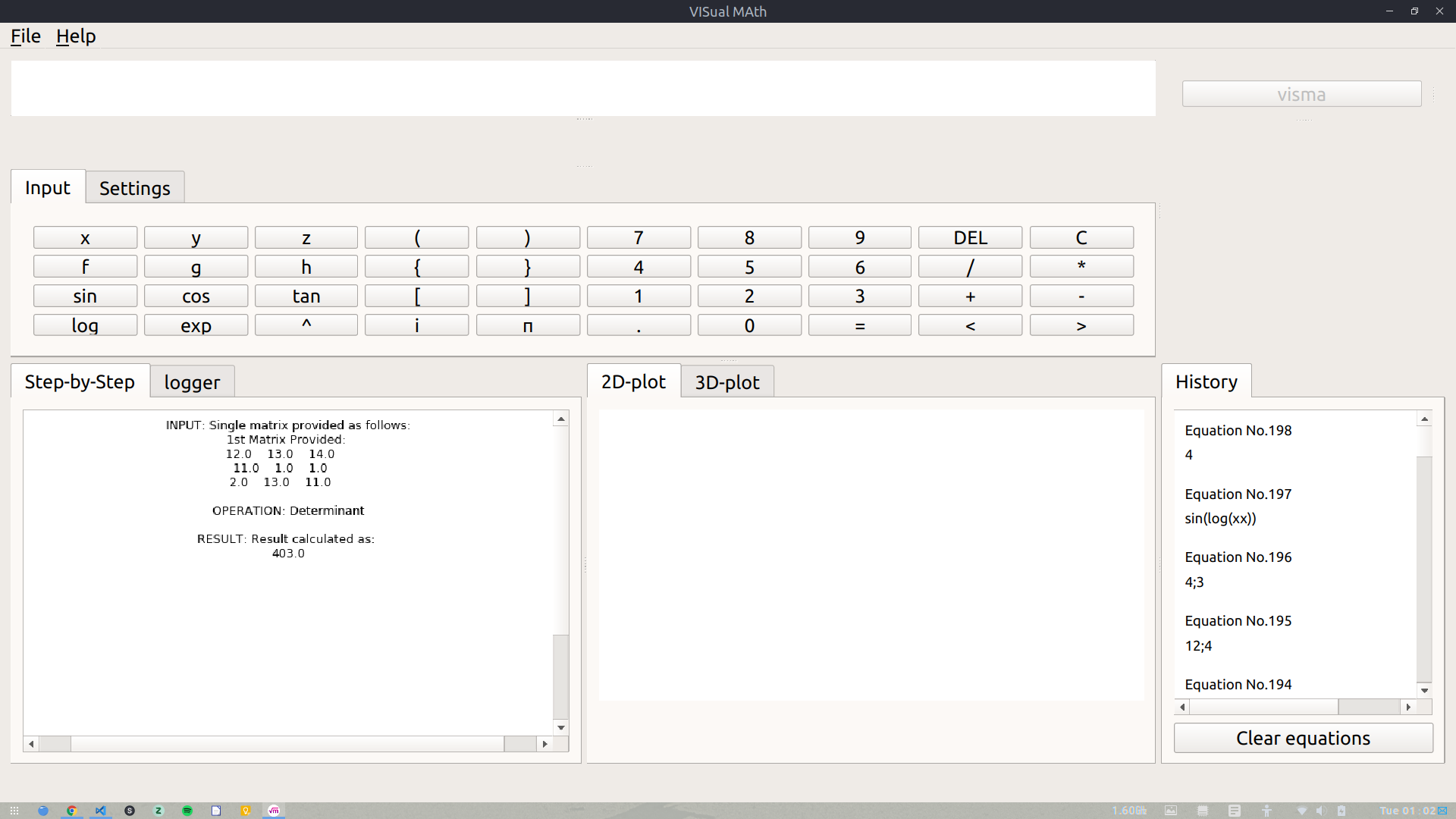
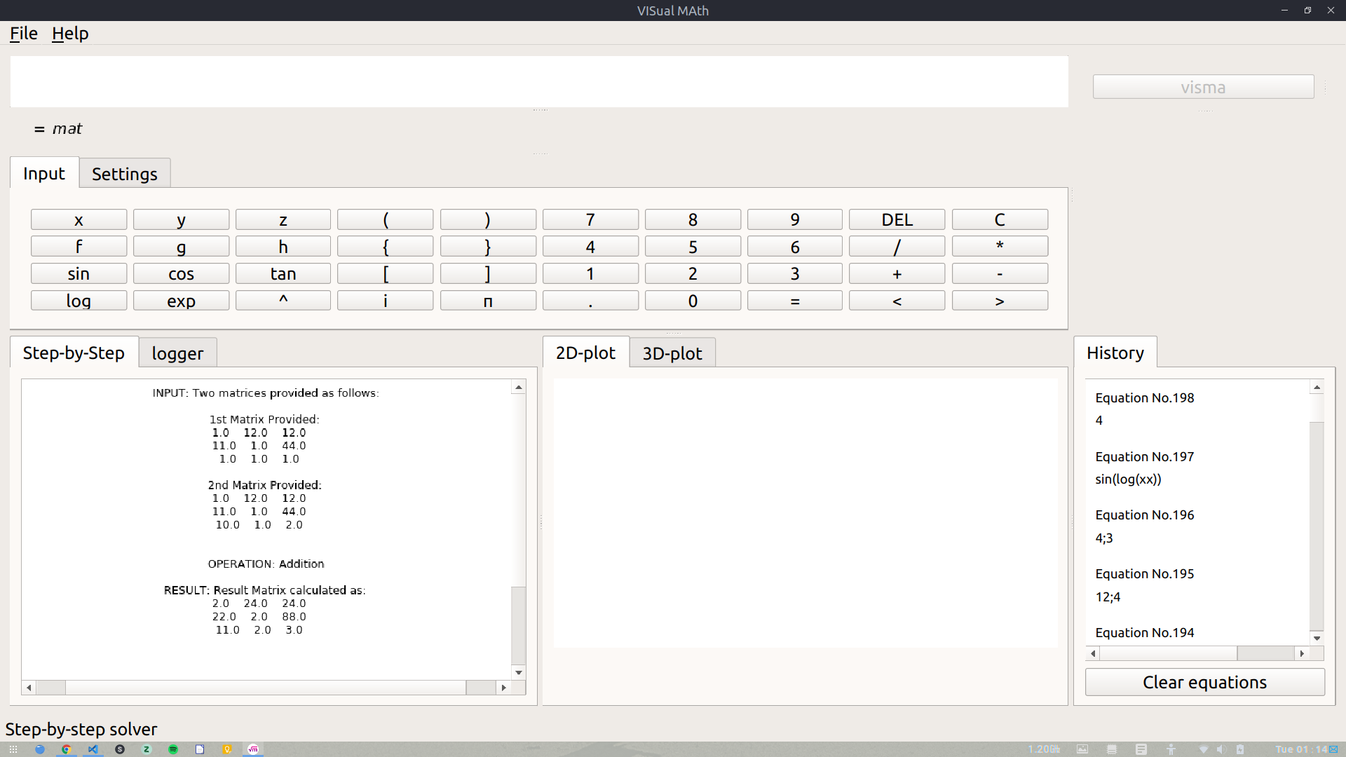
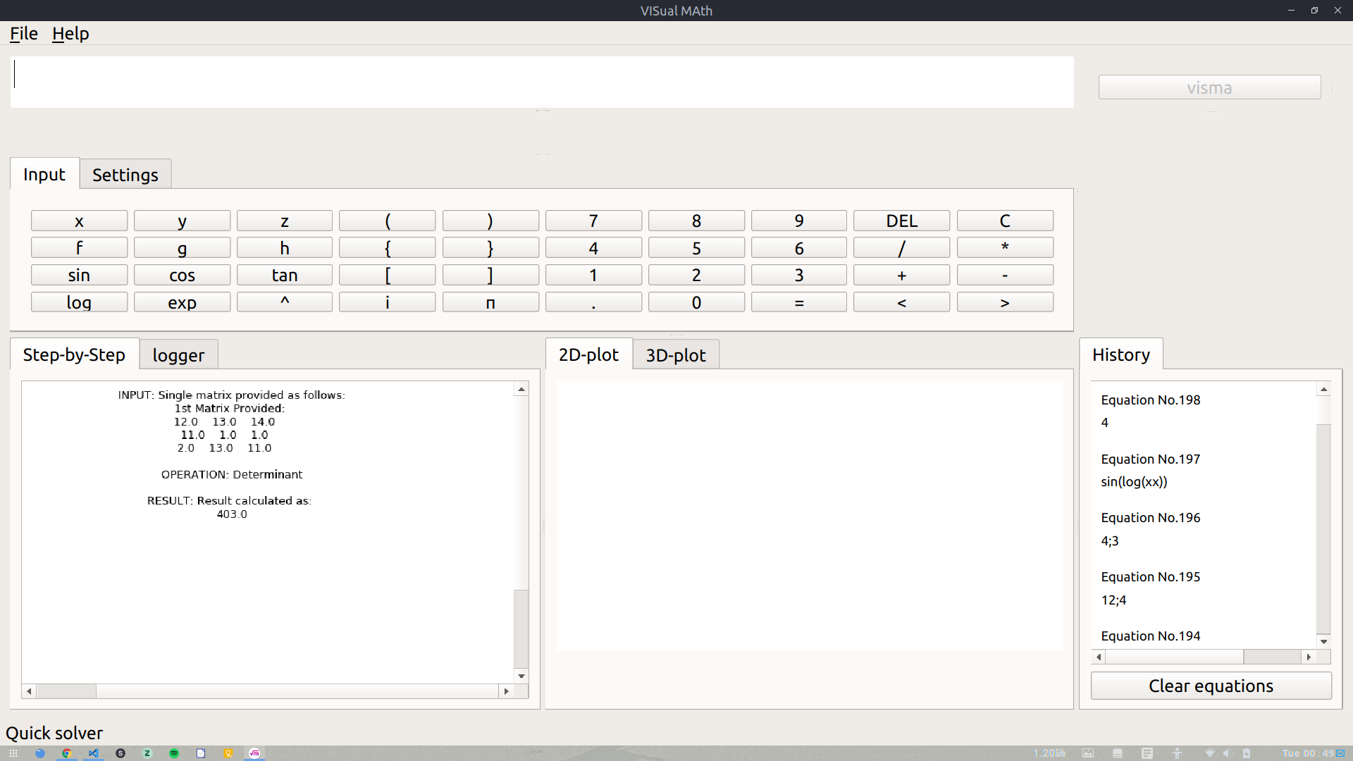
visma-VISualMAth, an equation solver and visualizer, which aims at showing the step-by-step solution & interactive plots of a given equation. As of now, VisMa is able to deal with matrices, multi-variable simultaneous equations & higher degree equations (up to four degrees) as well.
Via this blog, I will be giving a final wrap to everything I did during my wonderful stay at AerospaceResearch.net.
Before the start of GSoC 2019, following major deliverables were decided:
Re-writing simplify modules (addsub.py & muldiv.py) by using build-in class methods.
Adding support for Expression simplification
Adding a module for Discrete Mathematics
Adding support for equation solvers for cubic & biquadratic polynomials.
Adding support for simultaneous equations
Enhancing integration & derivation modules
Integrating matrix module with GUI
Rendering LaTex and Matplots in CLI
Including a Discrete Mathematics Module (including combinatorics, probability & statistics module)
All of the above-mentioned deliverables have been implemented. The commits referencing these changes are available at this link.
Below GIF shows the now integrated CLI module in action:
Some images showing matrix operations with VisMa are as follows:
Adding new modules & improving old ones was a great learning experience. Bugs were sometimes annoying however, each bug resulted in learning something new. That pretty much sums up all I did during GSoC.
I have written a developer blog for each of the Phases of GSoC, they are available as follows:
During the previous coding periods the key functionality
that was planned for this project was implemented. Thus, during the final
coding period there was time for improvements, development of one additional
feature whose inspiration came up during the previous period, refactoring and
organizing the file structure of the code as well as documenting the implemented
tool for feature users or developers.
First, the
following improvements were made:
-) The way
in which the minimum and maximum value of a continuous degree-of-freedom is
calculated was adjusted. Previously the minimum and maximum value was
calculated from the aggregate of the evolution data, which includes all lineages
and generations of the genetic optimization process. Now these values are
calculated specifically for each visualization scenario, only from the relevant
lineages and generations according to user defined options.
-) The part
of the code responsible for generating the animations was refactored and
extended to include the option to save the animations as compressed gif files.
The need for this arose after finding that the size of the gif files would
easily grow to tenths of megabytes even for the simple optimization scenarios
examined here.
Next, an
additional type of graphic, which allows for the visualization of useful
subsystems’ information on top of the existing 2d or 3d visuals was
implemented. This is a stacked bar graph spanning the y-axis on the 2d plots
and the z-axis on the 3d plots. The units of the stacked bar graphs are the
same as the units of the corresponding axis that it’s spanning. The height of
the individual bars of a stack are proportional to the values of the
corresponding degree-of-freedom of the respective subsystems that each bar is
representing.
Currently,
the stacked bar graphs are used to visualize the distribution of the electric
propulsion system’s total mass fraction into the corresponding subsystems.
Thus, the stacked bar graphs can be used to explore how the mass fraction of
each individual subsystem is changing as the genetic algorithms navigates
through different design points. To better understand this, let’s explore two
examples.
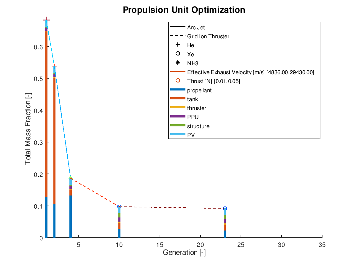
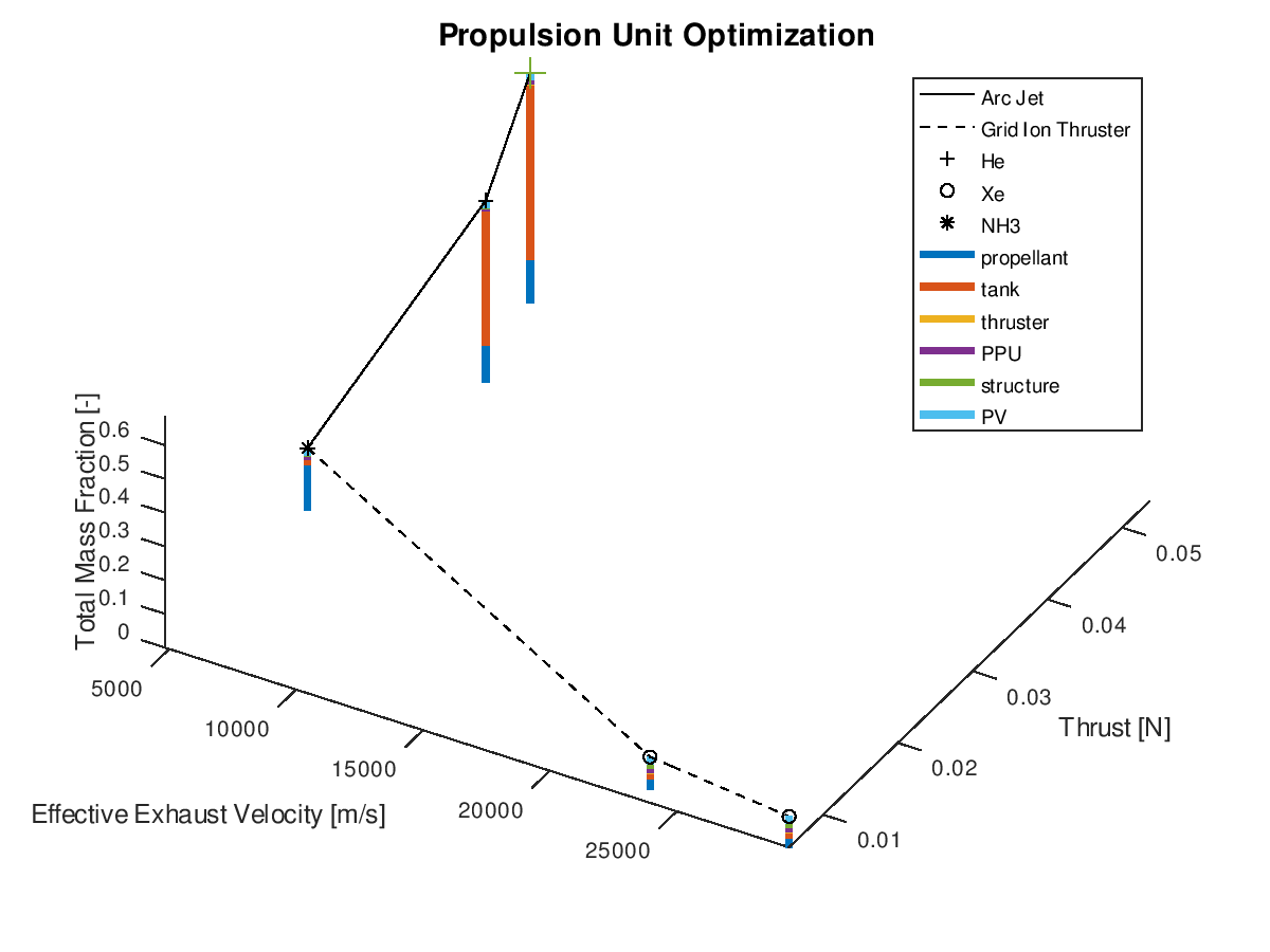
The first example is a 2d visualization, where the y-axis has been assigned to total mass fraction, the line style to propulsion system type, the line color to effective exhaust velocity, the marker to propellant and the marker color to thrust. Additionally, the stacked bar charts have been activated. As the y-axis corresponds to the total mass fraction, each bar of the stacks will correspond to the mass fraction of the respective subsystem. Only the best lineage is selected for visualization. The visualization system returns the following figure:
In the
figure above, we can examine how the mass fraction of each subsystem evolves as
the design of the system becomes optimal. In this simplified example, we can
see that the majority of the decrease of the total mass fraction can be
attributed to the reduction of the propellant and tank subsystems. Of course,
for this shrinkage to happen and the electric propulsion system to be able to
achieve the mission requirements, additional adjustments in other aspects of
the systems are being made by the optimization algorithm. Specifically, between
the starting and the final design point we can see that the propulsion system
type changes from Arcjet (solid line) to Grid Ion Thruster (dashed line), the
propellant changes from He (crosshair marker) to Xe (circle marker), the
effective exhaust velocity is increased (line color turns deep red from light
blue and “jet” is the chosen colormap) and the thrust is decreased (marker
color turns deep blue from deep red and “jet” is the chosen colormap).
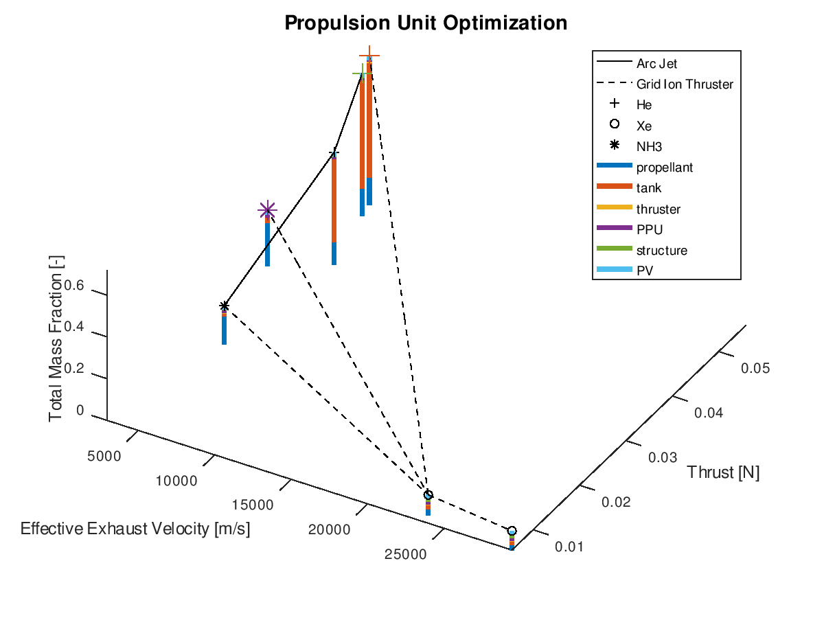
The stacked bar graphs can also be activated in 3d visualizations. In this next example, the x-axis has been assigned to effective exhaust velocity, the y-axis to thrust, the z-axis to total mass fraction, the line style to propulsion system type and the marker type to propellant. Only the best lineage is selected for visualization. The visualization system returns the following figure:
Like the
previous example, it’s easy to point out that the reduction of the total mass
fraction can be greatly attributed to the reduction of the propellant and tank
subsystems.
When using the stacked bar graphs in the 3d plot, it is also practical to include more lineages in the visualization. Selecting the three best lineages, the visualization system returns the following figure:
After this
final feature was implemented, additional refactoring of the code was done to
simplify certain parts and achieve improved extendibility and readability.
Refactoring the code was also done to end up in a restructured organization of
functions into subfolders. As the visualization system was designed with
flexibility, modularity and extendibility in mind, it is consisted of more than
100 functions. For this reason, a function dependency graph proved a great aid
for understanding the existing dependencies and making the appropriate
refactoring and restructuring decisions.
Finally, additional
documentation was created for this project to accompany the blog posts during
GSoC. All details regarding the available options and settings for configuring
the visualization system according to specific needs can be found in the
documentation. There, one can also find ready to use XML input file templates
which correspond to the visualizations found in all GSoC blog posts.
Congratulations
if you ‘ve made so far, this was the last long post! A final report will also
be released very soon!
This Project for this year’s edition of Google Summer of Code was titled: Decoding of ADS-B(Automatic dependent surveillance—broadcast)and Multi-lateralPositioning.
The aim of the project is to decode ADS-B frames/messages from raw IQ streams recorded using RTL-SDR radios and extract the data from these frames such as aircraft identifications, position, velocity, altitude etc.
The next part is to find the location of an aircraft when it sends a frame not having any position data in it’s payload using multilateration.
What is Multilateration ?
Multilateration is a method by which the location of an aircraft (can be any moving object which broadcasts a signal) using multiple ground stations and the Time Difference of Arrival(TDOA) of a signal to each ground station.
Implementations
Identification of long(112 bit) and short(56 bit) frames.
With the long frames, identifying each type of frame and the data contained in it.
Decoding and extracting the available data in the payload according to the frame type.
Building and outputting JSON files containing ADS-B frames and decoded data. (Gzipped)
Loading of files from multiple stations simultaneously.
Checking and grouping files which were recorded during the same time or have overlapping recording intervals.
Searching unique signals/frames in the overlapping files across different stations.
Testing
Since, position is one of the key component to this project, the first phase of testing was aimed at finding any hidden logical bugs in the code which calculates the position from the position containing frames.
As mentioned in the previous blogs, two methods are used to calculate the location.
The result obtained:
The plots in ‚yellow‘ are obtained from 3rd party trusted sources. This is a comparison plot of ‚our‘ output with trusted sources.
The project is expected to process files from several stations (5 stations) together. Thus there was a requirement to find files from different ground stations which were recorded at the same time interval. It can also be that the a part of the file overlaps. After which the ‚unique‘ frames were searched in these files.
The file overlap checker was tested with recordings from 5 stations recorded on 16th February in Germany.
This test run could find ‚unique‘ frames which were occuring atmost thrice, present at different ground stations.
Foremost, I would like to extend my sincere gratitude to my mentor and organisation head Andreas Hornig, for mentoring me throughout the season. Since I am not pursing a major in Computer Science altough coding and so called ‚cool stuffs‘ is my second hobby and passion, I would also like to appreaciate the additional energy and effort he has put in guiding me.
Besides, I put forth my vote of thanks to the organisation (Aerospaceresearch.net) as a whole, all the other mentors and the fellow students for making this organisation what it is and providing me with the opportunity to work on an open-source project.
In this blog post, I will be summarising all the work done during phase III (i.e. last phase of GSoC 2019).
This phase the major target was to wrap up all the work done during Phase I and Phase II. The first target was to implement GUI & CLI in matrices. The integration of GUI & CLI in matrices was pending from a long time and this was the time to get it done. The integration, however, was a bit tricky as it was very obvious that the usual parsers and tokenizers could not be used to integrate Matrices with GUI/CLI. We had to make an entirely new module which would be able to parse matrices (i.e. accept them as some input from the user and perform operations accordingly on them). We finally were able to properly integrate this module in GUI/CLI. It was worth the time & patience as the results were good. For now, the user has to enter the matrices in some specific Python list type pattern. In later versions, we can add options for adding matrices interactively by GUI.
Some screenshots of Matrix Module in action are:
The next part was adding test cases for Statistics modules (which were implemented during Phase II). Also, we added Equation Plotting feature in CLI during this part. It involved creating another Qt window equivalent to the plotter used in GUI version.
The last target of this phase was to add code to deal with cases when the Constant was raised to some fractional or Expression power. Earlier VisMa was able to handle only those cases when power was some Integer. The solution to this problem was to consider all the exponents as some object of Expression Class. Now since Expression simplification was done earlier this could be achieved. Also, I added the cases when Expression classes are involved in the Equation inputted by the user. Finally, our last target was to add the necessary documentation so that new users can get comfortable with the codebase. Personally, when I started to contribute to the project I found a lot of help because of docstrings & comments. Earlier developers (My mentors) have maintained a very well documented codebase, so it was my responsibility to carry this tradition forward.
To sum up, all the work done I am updating a list of all that we achieved during GSoC. The Changelog is as follows:
1. Simplify module written in Object-Oriented Programming Design.
2.__add__, __sub__ ,__mul__ & __truediv__ methods for most of the classes (like Constant, Expression, Trigonometric etc) have been added.
3. Discrete Mathematics Module has been added: a. Combinatorics modules like Combinations, Permutations & Factorial modules (with GUI/CLI implementations) b. Statistics Module containing mean, median and mode c. Simple probability modules d. Bit-wise Boolean Algebra module
4. Simultaneous Equation solver has been implemented
5. The plotter is now able to plot in both 2D and 3D for equations having one, two or three variables. It has been implemented in the CLI version
6. Equation solvers for higher degrees (Third & fourth degree) using determinant based approach have been added.
7. Integrations and differentiation modules are now implemented in all Function Classes (Trigonometry, Exponential and Logarithmic)
8. Integration & Differentiation modules have been rewritten to follow Object-Oriented Style.
9. Product Rule for Differentiation & Integration by parts module has been added.
10. Tokenize module is now improved to consider power operator (earlier it ignored power operator in many cases)
11. With above improvement Expressions raised to some power are duly handled by VisMa.
12. Parsing modules for printing matrices in Latex and string form have been added. With this matrix operations are now well implemented in GUI & CLI.
13. Expression simplification is now completely supported by VisMa. Almost all cases of Expression classes being involved in input equation have been taken care of. Multiple brackets are now also taken care by VisMa (for this the modules using recursion have been implemented).
14. The cases where Constant are raised to some fractional power or some solvable term have been covered.
The points where we will be working now are:
1. We can implement an Equation Scanner in the project. This way a user will be able to scan an image of the equation and it will be solved by VisMa. This was an idea during this GSoC but due to time constraints, we were not able to work in it for now.
2. VisMa is not friendly with Trigonometric expressions, there is a need to deploy some code in simplification module for taking care of this thing.
Overall, working in this community as a GSoC student was a great experience. It was hard but fun to stay within deadlines, fixing bugs, deploying new ideas etc. Feel free to connect with me on Twitter (https://twitter.com/mayank1Dhiman) & GitHub (https://github.com/mayankDhiman).
I discussed about how I am decoding the position of the aircraft from 2 ADS-B frames and also from 1 ADS-B frame and a reference position and how I found both handsome and erractic readings.
Let’s look into how other airborne parameters, such as ‚aircraft identity‘ and ‚velocity‘ are being decoded and calculated.
There is a special type of frame which is known as ‚Enhanced Mode-S‘ frames. They also contain similar information at times like the non-Enhanced Mode-S frames. I will elaborate on both in this blog.
Frames with downlink format 20 & 21 are known as Enhanced Mode-S frames.
The following methods were implemented in the code for decoding the information from the ADS-B frames.
Aircraft Identification
Frames with Downlink Format 17-18 and Type Code 1-4 are known as aircraft identification messages.
The structure of the 56-bit DATA field of any such aircraft identification frame will be as follows:
TC
EC
C1
C2
C3
C4
C5
C6
C7
C8
5
3
6
6
6
6
6
6
6
6
TC: Type Code
EC: Emitter Code
Second row signifies the bit-length
The EC value with regard to the TC value determines the type of aircraft (Such as : Super, Heavy, light etc). When the EC is set to ‚zero‘ signifies such information is not being transmitted by the aircraft.
An Airbus A380 is known as 'Super' and a Boeing 777-300ER is known as 'Heavy'. Small, private or training aircrafts such as Cessna 172s are known as 'Light'.
For determining the callsign a lookup table is used:
‚#‘ signifies a null value and ‚_‘ signifies a space between two words.
Let us take an Aircraft identifier frame recorded by one of our ground stations:
a0001910200490f1df2820700716
Thus the DATA part of this frame is:
200490f1df2820
BIN
00100000
000001
001001
000011
110001
110111
110010
100000
100000
INT
4
1
9
3
49
55
50
32
32
CHAR
[TYPE CODE]
A
I
C
1
7
2
_
_
The integer number corresponds to the corresponding element in the lookup table array.
Thus, the decoded callsign is „AIC172“ which belongs to Air India on the route 172
BDS 2,0 frames are also known as Aircraft Identification Messages. In these frames the first 8 bit of the DATA segment contains the BDS number and the rest is same as the previous one.
Airborne Velocity
ADS-B frames with Downlink Format 17-18 and TC 19 contain the velocity information of the aircraft.
Subtype 1 (Ground Speed)
The typical structure of the frame:
Position in frame
Position in data block
Length
Abbreviation
Data
33 – 37
1 – 5
5
TC
Type code
38 – 40
6 – 8
3
ST
Subtype
41
9
1
IC
Intent flag
42
10
1
RESV_A
Reserved-A
43 – 45
11 – 13
3
NAC
Velocity uncertainty (NAC)
46
14
1
S_ew
East-West velocity sign
47 – 56
15 – 24 change
10
V_ew
East-West velocity
57
25
1
S_ns
North-South velocity sign
58 – 67
26 – 35
10
V_ns
North-South velocity
68
36
1
VrSrc
Vertical rate source
69
37
1
S_vr
Vertical rate sign
70 – 78
38 – 46
9
Vr
Vertical rate
79 – 80
47 – 48
2
RESV_B
Reserved-B
81
49
1
S_Dif
Diff from baro alt, sign
82 – 88
50 – 56
7
Dif
Diff from baro alt
These two bits determine the direction at which the aircraft was flying:
S_ns:
     1 -> flying North to South
     0 -> flying South to North
 S_ew:
     1 -> flying East to West
     0 -> flying West to East
The speed and the heading can thus be computed by:
If the calculated heading is negative, then we add 360 to it.
Vertical Speed
The S_Vr bit (69) determines the direction(ascent/descent).
0- Up
1- Down
Therefore the actual speed is calculated by:
V = (int(Vr) – 1) * 64
Therefore, V is the speed and S_Vr states whether the aircraft is climbing or descending.
The VrSrc field (Vertical Rate Source) determines the measured altitude type:
Here let us see how the structure of Subtype 3 differs from Subtype1:
Position in frame
Position in data block
Length
Abbreviation
Data
33 – 37
1 – 5
5
TC
Type code
38 – 40
6 – 8
3
ST
Subtype
41
9
1
IC
Intent change flag
42
10
1
RESV_A
Reserved-A
43 – 45
11 – 13
3
NAC
Velocity uncertainty (NAC)
46
14
1
S_hdg
Heading status
47 – 56
15 – 24
10
Hdg
Heading (proportion)
57
25
1
AS-t
Airspeed Type
58 – 67
26 – 35
10
AS
Airspeed
68
36
1
VrSrc
Vertical rate source
69
37
1
S_vr
Vertical rate sign
70 – 78
38 – 46
9
Vr
Vertical rate
79 – 80
47 – 48
2
RESV_B
Reserved-B
81
49
1
S_Dif
Difference from baro alt, sign
82 – 88
50 – 66
7
Dif
Difference from baro alt
Heading
The S_hdg bit shows whether heading data is available or not:
0 - Heading data not available
1 - Heading data available
If heading data is available then it is calculated by:
Heading = Hdg(10 bit data) * 360/1024
Velocity (Airspeed)
Simply converting the AS bits gives the airspeed in knots.
Vertical Rate is calculated in the same manner as in Subtype 1
Enhanced Mode-S:
Aircraft Intention (BDS4,0)
The structure:
Field
Position
Length
Status
1
1
MCP selected altitude Precision = 16ft
2-13
12
Status
14
1
FMS selected altitude Precision = 16ft
15-26
12
Status
27
1
Barometric setting (in mb and not hPa) Value is actual minus 800 Precision = 0.1mb
28-39
12
Reserved
40-47
8
Status
48
1
VNAV hold state
49
1
ALT hold state
50
1
APP hold state
51
1
Reserved
52-53
2
Status
54
1
Altitude source: 00: Unknown 01:Aircraft altitude 10: MCP set altitude 11: FMS set altitude9
55-56
2
Note: MCP stands for Mode Control Panel where the pilot feeds in the data to the autopilot
FMS stands for Flight Management Computer where the data is fed to calculate various other flight parameters.
Track and Turn (BDS 5,0):
Many more information is given such as roll angle, true track angle etc:
Field
Position
Length
Status
1
1
Sign, 1
1
1
Roll angle range = [-90, 90] degrees Precision = 45/256 degree
3-11
9
Status
12
1
Sign
13
1
True Track angle Precision: 90/512 degree-
14-23
10
Status
24
1
Ground Speed Precision: 2 knots
25-34
10
Status
24
1
Sign
36
1
Track angle rate Precision: 8/256 degree/second
37-45
8
Status
46
1
True Airspeed Precision: 2 knots
47-56
10
Note: The sign bit determines whether to use 2's complement to determine the value present after it. It it is set to '1' then we have to use 2's complement.
Airspeed and Heading (BDS 6,0)
A lot more information is conveyed in this kind of frames:
Unfortunately the percentage of decodable Enhanced Mode-S message received was very low in both short recordings and long recordings which was worth hours.
File overlap checker:
The ground stations were programed to span each recorded file for 2 minutes(approx.). Now this means that for a long duration, there will be an array of files from several ground stations.
There has to be a logic, where the code finds all the files from several ground stations recorded at the same or has overlapping recording times and club them together for the next step.
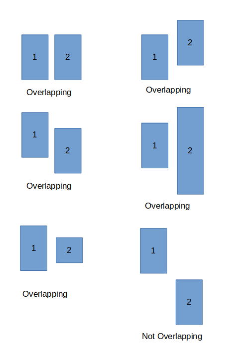
I identified few such cases of overlaps:
The overlapping files are clubbed together into a list for further processing.
Next step is to find the same frames present in different station recordings, so we need to know the files that overlap and process it accordingly.
In this blog, I will summarize all the work, that has been done during my three months of work at AerospaceResearch.net.
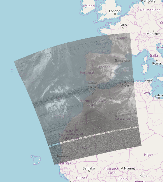
The resulting product is a fully functional web application and a set of supporting logic, that allows uploading, georeferencing, combining and displaying NOAA weather images. Below, more specific features are listed.
Work done
implemented functionality to extract and store satellite metadata
designed and implemented an accurate image georeferencing algorithm
designed and implemented an algorithm to merge several satellite images, taking care of overlapping areas
created CLI interfaces for each part of package API
implemented generation of web map and virtual globe
built custom web application, which includes web server backend with Flask and frontend
deployed the working application to the web (demo version at http://206.81.21.147:5000/map)
wrote tests, documentation, installation instructions and usage tutorials
For installation please see the installation guide in the repository description. To start using specific features please refer to the tutorials page, it contains usage examples with corresponding sample files for each use case. If you want to know more about how the software is working, please read my blogs. They describe in sufficient detail how the software is working.
Further work
Set up automatic data uploading from recording stations.
Set up a DNS domain.
Support
If you have any questions or issues concerning the usage of the software you can ask for help / open issues on GitHub or contact me directly.
This blog post will describe in general terms the architecture of web application, main steps of deployment process, processing server and several additional features.
General App Architecture
The application is an end-to-end data processing pipeline starting from raw satellite signal recordings and ending with displaying of combined images on the map or virtual globe. The image below describes this in a more structured way.
Figure 1. App architecture.
As showed on the image, the app consists of 4 main parts:
Recording stations
Processing server
Web server
Frontend
Data is being passed along this processing chain. Functionality of each part will be described in following parts of the article.
Processing Server
The task of processing server is to gather the raw satellite signal recordings and transform it to georeferenced images. This transformation happens using directdemod API:
DirectDemod decoder extracts the image from recording.
Image is preprocessed, two channels are extracted.
Each part is georeferenced and saved.
Processed data is being sent to web server.
Server uses ssh connection to securely transmit data, namely scp command is used. SCP stands for Secure Copy, it allows secure transmission of arbitrary files from local computer to remote machine.
Web Application
Web application is implemented using Flask. Web server has the following structure:
Figure 2. Web server.
It contains two main directories images/ – stores uploaded georeferenced image and tms/ – stores Tile Map Service representation of processed images. Images could be uploaded in two ways, either via ssh or throught /upload page (could be removed in production for safety reasons). After upload is done and the images are properly stored, then server will automatically merge this images using directdemod.merge and create TMS, which will be saved in tms/ directory. After processing is done, metadata will be updated and images will be displayed on website. Website itself contains 3 pages:
map.html
globe.html
upload.html (may be removed)
Map page displays images on Leaflet webmap, globe page uses WebGLEarth library to display images on Virtual Globe.
Should be noted that final implementation is somewhat different then showed on figure 2. Ability of viewing different channels was added, therefore tms stored in 2 directories corresponding to each channel.
Figure 3. Image of second channel.
Another major feature is called „Scroll in time“. Images are stored in chronological order and could be viewed sequentially using special slider. For each entry both channels could be viewed using a toggle button.
Deployment
Application has been deployed to the web http://206.81.21.147:5000/map. Appropriate domain name will be set up shortly.
Conclusion
This is the final part of the GSoC project. All main functionality and features have been implemented, web application is up and running.
In the previous blog, I penned down a brief introduction to ADS-B(Automatic Dependant Survelliance-Broadcast) and how this project has planned to have all the ground stations self-synchronised.
We now have the main data in our hand :- The ADS-B frames itself! Lets dive deep and see how I am extracting the data and what are the, both normal and non-normal, findings that I’ve made.
Findings
Starting with the first version of the my decoder and data extractor code, I tested it with a rather small, approximately 2 minutes long recording from one of the ground stations.
Before I discuss about what I found in the recording, here is an overview of what I had expected to be present in the recording and what are the capabilities of the current decoder file:
The structure of a typical ADS-B message with Downlink Format 17 when converted to its binary equivalent.:
Length
Position
Abbreviation
Name
5
1 – 5
DF
Downlink Format
3
6 – 8
CA
Capability
24
9 – 32
ICAO
ICAO aircraft address
56
33 – 88
DATA
Data
[33 – 37]
[TC]
Type code
24
89 – 112
PI
Parity/Interrogator ID
Length of the messages according to Downlink Format(DF):
112 bit (long): DF 16, 17, 18, 19, 20, 21, 22, 24
56 bit (short): DF 0, 4, 5, 11
Not all data is contained in a single message, here’s how to know what data is contained in a particular message based on the Type Code:
Type Code(TC)
Data
1 – 4
Aircraft identification
5 – 8
Surface position
9 – 18
Airborne position (Baro Altitude)
19
Airborne velocities
20 – 22
Airborne position (GNSS Altitude)
23 – 27
Reserved
28
Aircraft status
29
Target state and status information
31
Aircraft operation status
Now, the percentage of each type of message that I found in the recording:
Aircraft Identifiers: 0.77 %
Messages with surface position: 0.00 %
Airborne Position (Barometric Altitude): 8.21 %
Airborne Velocity messages: 7.60 %
Airborne Position (GNSS altitude): 0.00 %
Operation Status messages: 0.82 %
Enhanced Mode-S ADS-B data: 34.46 %
Squawk/Ident data: 3.09 %
Short Air to Air ACAS messages: 14.47 %
Encoded Altitude only: 29.22 %
Long ACAS messages: 1.34 %
A total of 13172 messages were detected in this recording.
After a brief analysis what I observed is, the velocity of each aircraft is sent almost after every 4-5 position messages. The reason for the absense of any surface position messages can be that the ground station was not close enough to any airfield. And, by looking at the statistics, usage of barometric altitude seems to be a standard than GNSS altitude.
Decoding the Data
Our prime point of focus are the Airborne Position messages (DF 17-18, TC 9-18) as the title of the project suggests. Let’s discuss about how my code goes about decoding the location from each frame.
Pre-Step : Creating ‚identifier‘ functions which determines the message type. One such identifier function would be an ‚Airborne Position‘ message identifier.
Typical structure of an ‚Airborne Position‘ Message is given as:
Airborne position message bits explained
Position
Position in Data block
Bit Length
Content
33 – 37
1 – 5
5
Type code
38 – 39
6 – 7
2
Surveillance status
40
8
1
NIC supplement-B
41 – 52
9 – 20
12
Altitude
53
21
1
Time
54
22
1
CPR odd/even frame flag
55 – 71
23 – 39
17
Latitude in CPR format
72 – 88
40 – 56
17
Longitude in CPR format
There are two methods of determining the location:
Globally Unambiguous method: This method requires two frames for the calculation. The frames should be a pair of an odd frame and an even frame, received in succession. Two even frames or two odd frames will not work in this method.
Bit-54 in the binary equivalent of the message is the flag bit that tells us whether the frame is even or odd.
0 – Even Frame
1 – Odd Frame
Bits 55-71 contain latitude in CPR format, and bits 72-88 contain longitude in CPR format. Thus the CPR is calculated by
LAT_CPR = decimal(bits 55-71) / 131072
LON_CPR = decimal(bits 72-88)/ 131072
The decimal equivalent of the CPR is encoded in 17 bits. So the maximum value that it can have is 2^17 or 131072, thus the CPR is mapped to a floating value below 1 by dividing it by 131072.
Calculation of Latitude:
Latitude Index(j):
We need two constants to compute the relative latitudes
Where NZ is the abbreviation of number of geographic latitude zones present between the equator and the poles. NZ = 15 is a standard for Mode-S position encoding.
Thus, the calculation of the relative latitude coordinate:
For locations in southern hemisphere, the latitude lies between 270 – 360 degrees, but we need to restrict the range to [-90, 90]
The final latitude is chosen based on the newest frame received. If the newest received frame has an even CPR flag, then the even latitude (LatEven) will be the final latitude and vice-versa.
We now have one coordinate in our hand !!
Before we place foot in computing the longitude, we should check if both the latitudes in the two frames are consistent, i.e. they lie in the same latitude zone
Check for Latitude zone consistency:
Let’s define a function which returns the number of latitude zones. ‚NL(latitude)‘ is how it is named.
NL():
The returned value lies in the closed interval [1, 59]
Both the calculated latitude of the even and the odd frames are passed to this function, if the returned value is equal for both the cases, then both of them lies in the same zone, and the code has successfully removed the ambiguity in them.
If the returned values are unequal, then skip the calculation and wait for a new message.
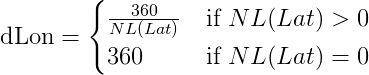
Calculation of Longitude:
If the newer message among the pair of frames is even:
When the newer message to be received is odd:
For both cases, if Lon is greater than 180 degrees
Now we have the coordinates of the aircraft (lat, lon) calculated using the ‚Globally unambiguous method‘
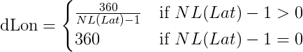
Locally unambiguous method:
This method requires a reference location for calculation. This location must be within 180NM from the location to be calculated.
Calculation of dLon
Latitude index (j):
Latitude is thus given by:
Calculation of longitude:
Here NL function is the same as it has been defined for the 'Globally Unambiguous method'.
Longitude index (m):
Thus, longitude is given by:
Calculation of Altitude:
Bits 41-52 contain the altitude in a DF 17 TC 9-18 ADS-B frame
Bit 48 is known as the Q-Bit which determines the encoding multiple of the altitude
If Q-Bit = 1; 25 feet
else if Q-Bit = 0; 100 feet
The binary string spans from bit 41-52 excluding Q-bit(48)
Thus the Altitude is given by:
Where N is the decimal equivelent of bit 41-52 excluding the Q-bit
It was now time to execute this implementation !!
And here are the first set of results:
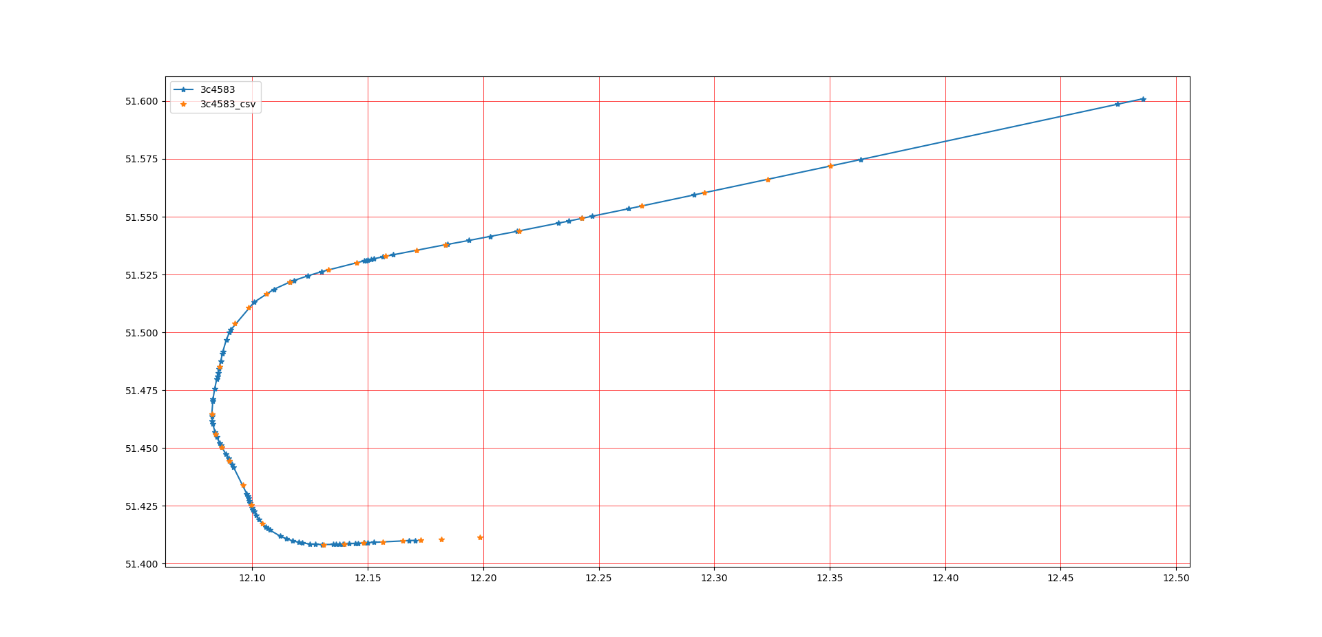
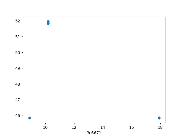
Here is a comparison of the results obtained from my code and data acquired from trusted 3rd party sources
The blue plots are the locations calculated by the current code.
Whereas, the yellow plots are the ones obtained from other sources.
The 3rd party sources do not give us with raw calculated data, that's why the plots do not match even though the flight path overlaps.
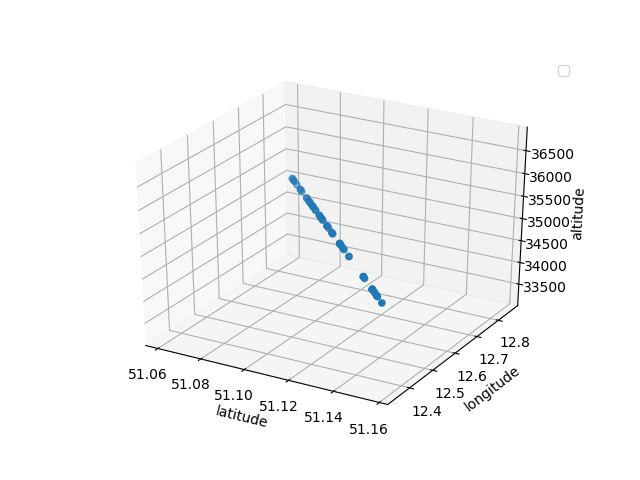
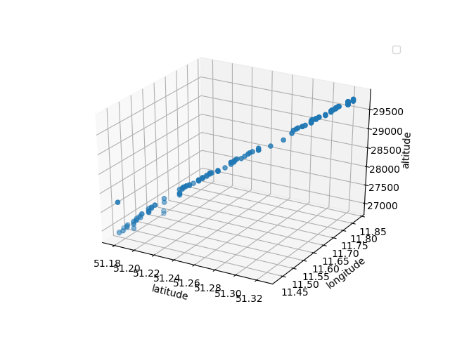
Here is a plot where you can identify a cruising aircraft:
And also an aircraft which is beginning is decent towards Leipzig Airport:
Unusual findings:
The first stage of the code where I had implemented the decoding of position only by ‚Globally Unambiguous Method‘, I found a few stray points in the plots. A good term for this would be removal of ‚Vomit Comets‘. For example:
As you can see, it does not define a proper flight path.
Here, I now introduce a checking system, where the position of the newest frame is calculated using the ‚Locally unambiguous method‘ and it then compares both the positions.
If there is a difference, then the position calculated by the latter method is taken as ultimate.
Also, many singular frames were skipped from the intial position calculation logic as there wasn’t a compatible succesive frame. For them, the location calculated by the latter method was final.
Up Next:
I will dig further into how I am decoding and calculating other flight parameters such as, airspeed, ground speed, heading, aircraft identify codes (such as SQUAWK and Callsign).
Also, the initial phases after the completion of the decoding layer: Searching of overlapping files from different ground stations.
This is the
second in a series of blog posts, where I am documenting the progress of my
project and my experience working with aerospaceresearch.net for Google Summer
of Code 2019.
Last time I
went into details about the often synonymous concepts, in the engineering world,
of designing and optimizing a system. The provided context served as a prerequisite
for explaining the purpose and the motivation behind both the KSat project, as
well as my contribution in the project, which is the development of an automated
visualization system to explore different design points, gain insights about
the optimization process and the genetic algorithm’s performance, aid in
debugging and more. In case you missed it and you would like to have more
information, you can find the first blog post here: https://aerospaceresearch.net/?p=1542
. In fact, I highly recommend that you have read the first blog post before
moving on with the second one.
From this point on, this blog post will focus on the
progress during the second coding period. Before I get into technical topics,
since I am documenting the whole experience, I would like to write a couple of
words about the collaboration and the communication within aerospaceresearch.net.
Like mentioned in the first blog post, everyone inside the organization has
been extremely welcoming and helpful even from the pre-application stage. As it
is to be expected during the second coding period, I was even more familiar
with my project as well as with the exact fit of my work in the bigger picture.
The communication with my main mentor, Manfred, continues to take place in an
almost daily base for anything related to my work and I would like to thank him
one more time for his valuable input and our great collaboration.
Regarding the technical aspects of my project, attention was first given in making the visualizations more presentable and readable. For this purpose, the structure of the xml that serves as an input to the visualization system, was extended to accommodate the following functionality:
-) Application of custom axes limits or limits that are
calculated from the optimization data.
-) Definition of viewing angle for the 3d plot.
-) Definition of plot title.
-) Definition of axes labels that correspond to
degrees-of-freedom (DoFs) that are assigned in x-, y- and z- axis.
-) Definition of legends that correspond to DoFs that are
assigned in line style and line color as well as marker and marker color.
Some additional options like defining the font size for the
title, the labels and the legends are available. The above functionality is more
or less self-explanatory, but in order to make things more tangible the
following visualizations from the first blog post are presented. The difference
here is, that the visualizations have been properly annotated by activating the
corresponding options through the xml file.
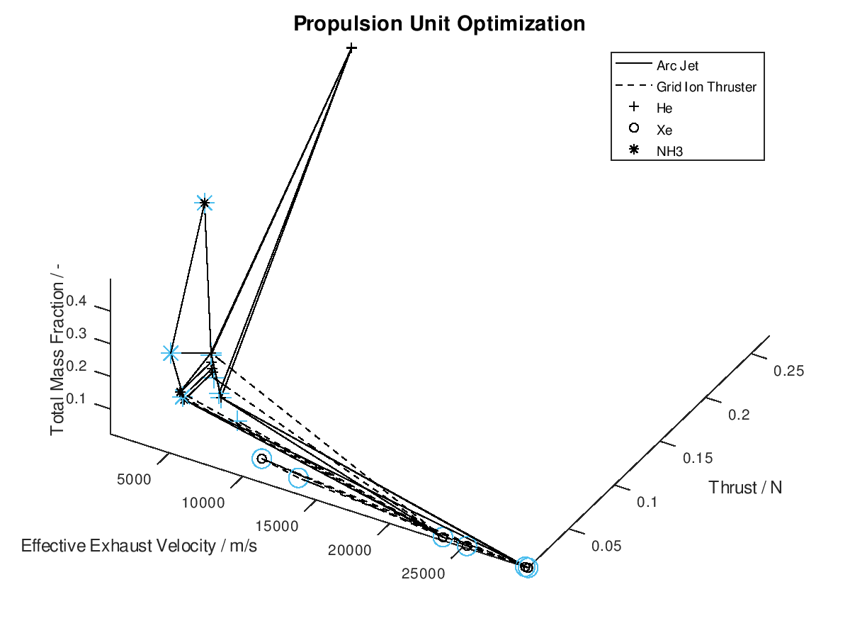
The first visualization from the first blog post, would take the following form:
In the figure above, I have defined “Propulsion Unit Optimization” as the title to applied on the plot as well as “Effective Exhaust Velocity / m/s”, “Thrust / N”, and “Total Mass Fraction / -“ as the labels of the x-, y- and z- axis correspondingly. In addition, I have specified that the axes limits should be calculated from the optimization data and that the viewing angle should be [azimuth, elevation] = [30, 60]. I have also enabled the legend for the remaining of the activated DoFs, which in this case are propulsion type and propellant. As it can be seen on the legend, propulsion type (arc jet or grid ion thruster) has been assigned to line style (solid or dashed), while propellant (He, Xe or NH3) has been assigned to marker (crosshair, circle or star). The chosen font sizes in this example are 14 for the title, 12 for the labels and 9 for the legends. At this point it should be noted that some of the above options, concerning the appearance of the visualization, were also manually applied at the corresponding visualization of the first blog post. The difference here is, that their automatic application has now been implemented as a series of activatable options in the xml file.
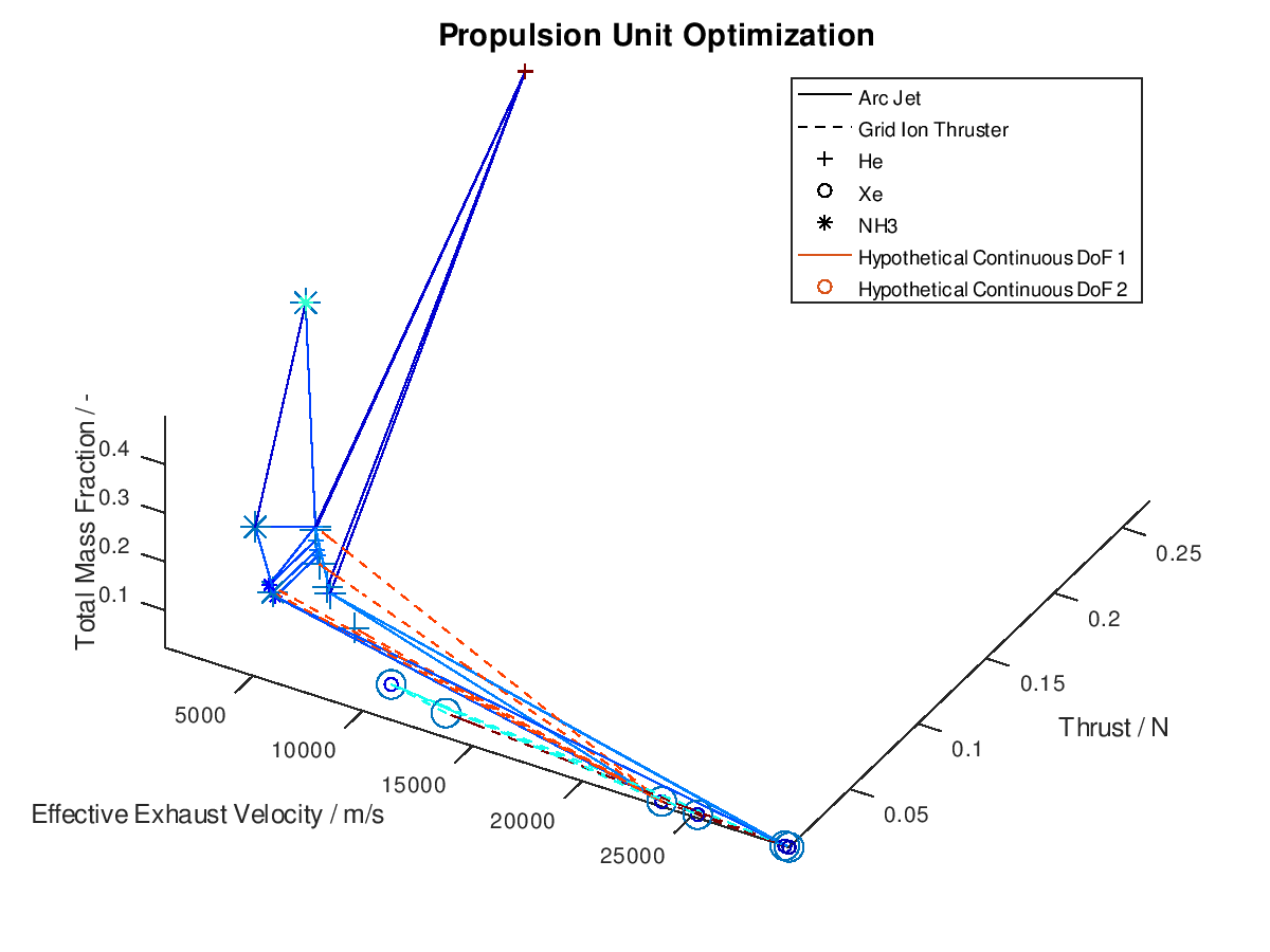
Now that we have an idea about the way in which the majority of a visualization’s elements are annotated, lets also see how potential additional continuous DoFs that are assigned to line and marker color are presented. For this purpose, we are going to use the last visualization from the first blog post, which would take the following form:
The difference in this visualization compared to the
previous one is, that two additional hypothetical continuous DoFs have been assigned
to line and marker colour. To indicate this, the corresponding DoFs “Hypothetical Continuous DoF 1” and “Hypothetical
Continuous DoF 2” are included in the legend with a colored line and mark. Notice
that are all other elements in the legend are black. The colored elements
indicate that the value of these continuous dofs corresponds to the line and
marker color in the visualization.
Now that we have covered the annotation of the visualizations, lets move to the remaining implemented functionality. A second type of visualization, a 2d visualization, was added in the visualization system. The motivation for the 2d plot is similar to the motivation for the 3d plot. Different system DoFs can be assigned to y-axis, line style and color as well as marker style and color. Notice that the x- and z-axis are no longer available to the user. At this point you may ask what the purpose of the 2d plot is then. In the 2d plot the x-axis corresponds to the generations of the system’s evolution, thus the 2d plot can be used to acquire a clearer picture regarding the chronological order in which different lineages evolve through different design points.
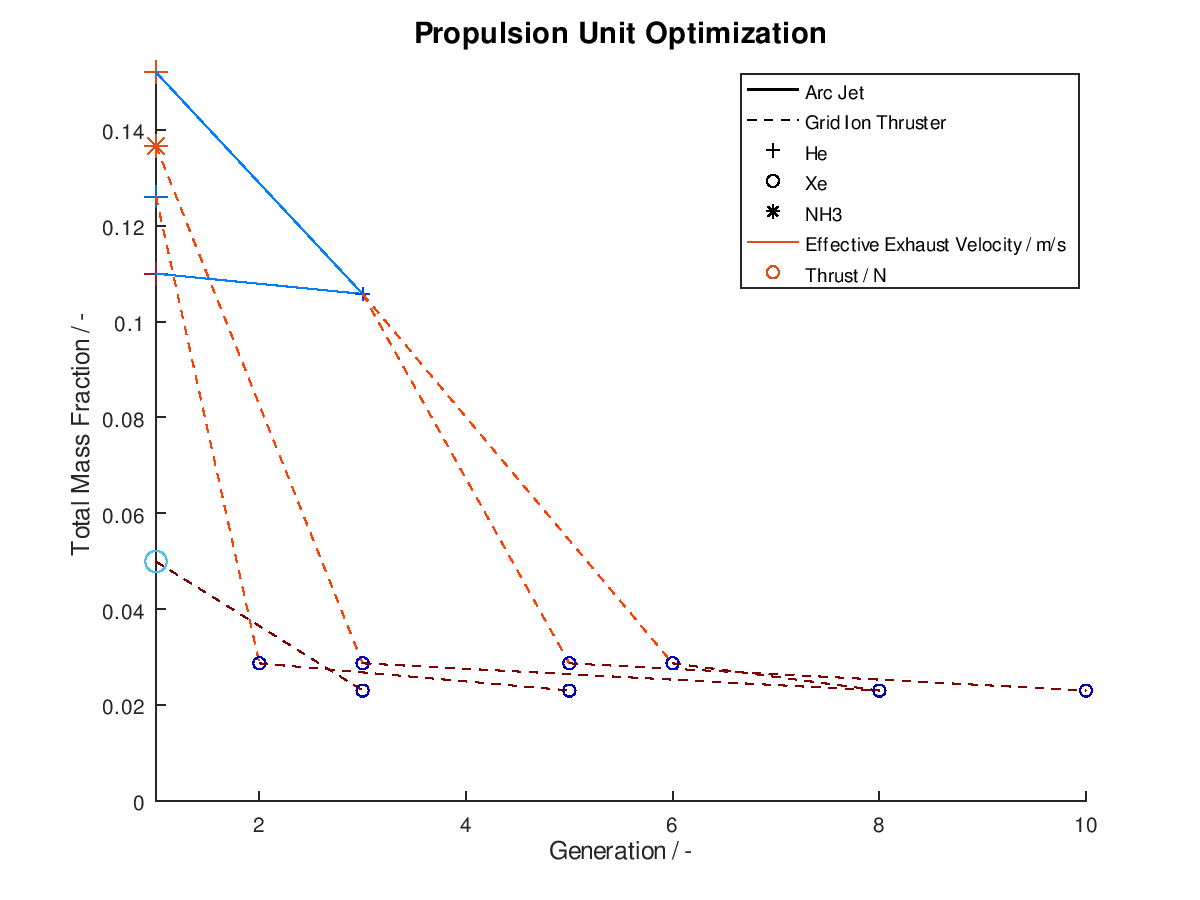
As usual I am going to give a practical example. I assign total mass fraction to y-axis, propulsion type to line style, propellant to marker, effective exhaust velocity to line color and thrust to marker color. I deactivate the visualization of failed mutations, I sort the lineages by total mass fraction and I keep only the 5 best lineages. I also activate the use of the implemented annotations. The plotting system returns the following figure:
As we can
see from the figure above, all lineages converge to almost identical final design
points. One lineage achieves this in just 3 generations, while another one need
as much as 10 generations. In between of improved design points, we can also observe
the number of generations where failed mutations occurred. For the lineage that
converges on the 10th generation we can see that the successful mutations
take place at the 3rd, 6th and 10th generation.
This means that the mutations of the generations 2, 4-5 and 7-9 were failed
mutations.
Another
implemented feature is the ability to save the generated visualizations in a
desired file format. This is required in order to review the progress of the
optimization process after the execution of an optimization cycle. For this purpose,
the following functionality was implemented as an activatable option through
the xml file.
-) Saving
of the visualization in one or more file formats. The available file formats
are: *.ps, *.eps, *.jpg, *.png, *.emf, *.pdf
-) Generating
filenames according to input case number, input/mission parameters and plot
case number.
In order to
avoid loss of any generated visualization it is important that the generated
filenames always remain different regardless of the number of visualizations or
the activated filename options. For this purpose, a hard-coded fail-safe check
was also included. A sample generated filename could be “input_case_1_totalimpulse_112670_deltav_686_plot_case_1”.
In this case, the input case number, the mission parameters (total impulse and velocity
increment) along with their corresponding values and the plot case number, were
all included in the title. For distinction purposes between different
visualizations the plot case number is always included in the title, while in
the absence of mission parameters the input case number is also automatically
included.
Finally, another way to reap more potential insights from the visualizations is to include the dimension of time in them. This was achieved to a certain extend with the use of the 2d plot where the x-axis corresponds to the generations. There is another way to do so, where the graphics objects that form the visualizations are animated through a series of frames that follow the evolution of the system that is being optimized. The output is a series of frames that form a gif animation, rather than a single snapshot. The graphics objects can be animated in two different ways.
According to the first approach, the graphics objects are animated separately for each lineage. The sequence of the design points that correspond to the best lineage are animated first, then those that correspond to the second best and so on. This animated version of the last visualization of the first post, is the following:
In the
animation above, only the 10 best lineages have been included. The frame rate
of the animation is defined at 2 fps through the xml file.
The other
way in which the graphics objects of a visualization can be animated, is for
all lineages together. In this case, the sequence of the design points of all selected
lineages is animated according to the progression of the generations. Design points that appear on the same frame
correspond to mutations of different lineages that took place on the same
generation during the optimization process. This animated version is the
following:
It should
be noted that the examples for which the animations were applied, are simplified,
thus a certain visual overlap occurs between different lineages. This causes
the animations to appear stagnant at times, while what is really happening is
that some lineages follow an identical sequence of design points as others. These
design points have already appeared in the visualization due to already
visualized lineages or due to lineages that have advanced through them at an
earlier generation, giving the illusion that the animation remains stagnant at times,
but this is not the case.
One final
thing to mention is, that not only a 3d plot but also a 2d plot can be animated
in a similar fashion.
Summing up
this second blog post, we got a brief overview as well as a quick demonstration
of the newly added features. We saw how these features build on top of the
existing ones and open the possibilities for further exploration of the
evolution data. There are some cases where minor bug fixes are required, and potential
improvements and extensions have already been identified. Documentation is also
going to be developed, but all that is work for the following weeks …
Congrats
for making it through the second blog post and many thanks for reading!